import xarray as xr
import xgcm
import numpy as np
import xroms
import matplotlib.pyplot as plt
Matplotlib is building the font cache; this may take a moment.
How to calculate with xarray and xroms
Here we demonstrate a number of calculations built into xroms, through accessors to DataArrays and Datasets.
xarray Datasets
Use an xarray accessor in xroms to easily perform calculations with syntax
ds.xroms.[method]
Importantly, the xroms accessor to a Dataset is initialized with an xgcm grid object (or you can input a previously-calculated grid object), stored at ds.xroms.xgrid, which is used to perform the basic grid calculations. More on this under “How to set up grid” below.
The built-in native calculations are properties of the xroms accessor and are not functions.
The accessor functions can take in the horizontal then vertical grid label you want the calculation to be on as options:
ds.xroms.ddz('u', hcoord='rho', scoord='s_rho') # to make sure result is on rho horizontal grid and s_rho vertical grid, a function
or
ds.xroms.dudz # return on native grid it is calculated on, a property
Other inputs are available for functions when the calculation involves a derivative and there is a choice for how to treat the boundary (hboundary and hfill_value for horizontal calculations and sboundary and sfill_value for vertical calculations). More information on those inputs can be found in the docs for xgcm such as under found under:
ds.xroms.xgrid.interp?
xarray DataArrays
A few of the more basic methods in xroms are available to DataArrays too. xroms methods for DataArrays require the grid object to be input:
ds.temp.xroms.to_grid(xgrid, hcoord='psi', scoord='s_w')
Attributes
xroms provides attributes as metadata to track calculations, provide context, and to be used as indicators for plots.
The option to always keep attributes in xarray is turned on in the call to xroms.
cf-xarray
Some functionality is added by using the package cf-xarray. Necessary attributes are added to datasets when the following call is run:
ds, xgrid = xroms.roms_dataset(ds)
For example, when all CF Convention attributes are available in the Dataset, you can refer to dimensions and coordinates generically, regardless of the actual variable names.
For dimensions:
ds.cf[“T”], ds.cf[“Z”], ds.cf[“Y”], ds.cf[“X”]
For coordinates:
ds.cf[“time], ds.cf[“vertical”], ds.cf[“latitude”], ds.cf[“longitude”]
Load in data
More information on input/output in input/output page. For model output available at
ds = xr.open_dataset(url, chunks={})
Also, an example ROMS dataset is available with xroms that we will read in for this tutorial.
ds = xroms.datasets.fetch_ROMS_example_full_grid()
ds
Downloading file 'ROMS_example_full_grid.nc' from 'https://github.com/xoceanmodel/xroms/raw/main/xroms/data/ROMS_example_full_grid.nc' to '/home/docs/.cache/xroms'.
<xarray.Dataset> Size: 62MB
Dimensions:     (eta_rho: 191, xi_rho: 300, s_rho: 30, ocean_time: 2, s_w: 31,
                 eta_u: 191, xi_u: 299, eta_v: 190, xi_v: 300)
Coordinates:
    lon_rho     (eta_rho, xi_rho) float64 458kB dask.array<chunksize=(191, 300), meta=np.ndarray>
    lat_rho     (eta_rho, xi_rho) float64 458kB dask.array<chunksize=(191, 300), meta=np.ndarray>
  * s_rho       (s_rho) float64 240B -0.9833 -0.95 -0.9167 ... -0.05 -0.01667
  * s_w         (s_w) float64 248B -1.0 -0.9667 -0.9333 ... -0.03333 0.0
  * ocean_time  (ocean_time) datetime64[ns] 16B 2009-11-19T12:00:00 2009-11-1...
    lon_u       (eta_u, xi_u) float64 457kB dask.array<chunksize=(191, 299), meta=np.ndarray>
    lat_u       (eta_u, xi_u) float64 457kB dask.array<chunksize=(191, 299), meta=np.ndarray>
    lon_v       (eta_v, xi_v) float64 456kB dask.array<chunksize=(190, 300), meta=np.ndarray>
    lat_v       (eta_v, xi_v) float64 456kB dask.array<chunksize=(190, 300), meta=np.ndarray>
Dimensions without coordinates: eta_rho, xi_rho, eta_u, xi_u, eta_v, xi_v
Data variables: (12/17)
    angle       (eta_rho, xi_rho) float64 458kB dask.array<chunksize=(191, 300), meta=np.ndarray>
    hc          float64 8B ...
    Cs_r        (s_rho) float64 240B dask.array<chunksize=(30,), meta=np.ndarray>
    zeta        (ocean_time, eta_rho, xi_rho) float32 458kB dask.array<chunksize=(2, 191, 300), meta=np.ndarray>
    h           (eta_rho, xi_rho) float64 458kB dask.array<chunksize=(191, 300), meta=np.ndarray>
    Cs_w        (s_w) float64 248B dask.array<chunksize=(31,), meta=np.ndarray>
    ...          ...
    temp        (ocean_time, s_rho, eta_rho, xi_rho) float32 14MB dask.array<chunksize=(2, 30, 191, 300), meta=np.ndarray>
    salt        (ocean_time, s_rho, eta_rho, xi_rho) float32 14MB dask.array<chunksize=(2, 30, 191, 300), meta=np.ndarray>
    Vtransform  int32 4B ...
    pm          (eta_rho, xi_rho) float64 458kB dask.array<chunksize=(191, 300), meta=np.ndarray>
    pn          (eta_rho, xi_rho) float64 458kB dask.array<chunksize=(191, 300), meta=np.ndarray>
    f           (eta_rho, xi_rho) float64 458kB dask.array<chunksize=(191, 300), meta=np.ndarray>
Attributes: (12/29)
    file:              ocean_his_0150.nc
    format:            netCDF-3 classic file
    Conventions:       CF-1.4
    type:              ROMS/TOMS history file
    title:             Texas and Louisiana Shelf case (Nesting)
    rst_file:          ocean_rst.nc
    ...                ...
    compiler_command:  /g/software/openmpi/1.4.3/intel/bin/mpif90
    compiler_flags:    -heap-arrays -fp-model precise -assume 2underscores -c...
    tiling:            016x032
    history:           ROMS/TOMS, Version 3.4, Sunday - December 4, 2011 -  7...
    ana_file:          /scratch/zhangxq/projects/txla_nesting6/Functionals/an...
CPP_options: TXLA, ANA_BSFLUX, ANA_BTFLUX, ASSUMED_SHAPE, BULK_FLUX...ds, xgrid = xroms.roms_dataset(ds, include_cell_volume=True)
# add grid to xrom accessor explicitly
ds.xroms.set_grid(xgrid)
ds.xroms.xgrid
<xgcm.Grid>
X Axis (not periodic, boundary=None):
  * center   xi_rho --> inner
  * inner    xi_u --> center
Y Axis (not periodic, boundary=None):
  * center   eta_rho --> inner
  * inner    eta_v --> center
Z Axis (not periodic, boundary=None):
  * center   s_rho --> outer
  * outer    s_w --> center
xgcm grid and extra ROMS coordinates
How to set up grid
The package xcgm has many nice grid functions for ROMS users, however, a bit of set up is required to connect from ROMS to the xgcm standardds. This grid set up does that.
The grid object contains metrics (X, Y, Z) with distances for each grid (‘dx’, ‘dx_u’, ‘dx_v’, ‘dx_psi’, and ‘dz’, ‘dz_u’, ‘dz_v’, ‘dz_w’, ‘dz_w_u’, ‘dz_w_v’, ‘dz_psi’, ‘dz_w_psi’), and all of these as grid coordinates too.
After setting up your Dataset, you should add coordinates and other information to the dataset and set up an xgcm grid object with:
ds, xgrid = xroms.roms_dataset(ds, include_cell_volume=True)
If you want to use the xroms accessor, add the grid object explicitly with:
ds.xroms.set_grid(xgrid)
If you don’t do this step, the first time the grid object is required it will be set up, though you can’t choose which input flags to use in that case.
The xgcm grid object is then available at
ds.xroms.xgrid
Grid lengths
Distances between grid nodes on every ROMS grid can be calculated and set up in the xgcm grid object — some by default and some have to be requested by the user with optional flags.
Horizontal grids:
inverse distances between nodes are given in an analogous way to distance (i.e.,
ds.pmandds.pn_psi)distances between nodes are given in meters by dx’s and dy’s stored in ds, such as:
ds.dxfor therhogrid andds.dy_psifor thepsigrid, calculated from inverse distancesVertical grids:
There are lazily-evaluated z-coordinates for both
rhoandwvertical grids for each horizontal grid.There are also arrays of z distances between nodes, called dz’s, available for each combination of grids. For example, there is
ds.dz_ufor z distances on theuhorizontal andrhovertical grid, and there isds.dz_w_vfor z distances on thevhorizontal andwvertical grid. These are[ocean_time x s_* x eta_* x xi_*]arrays.Arrays of z distances relative to a sea level of 0 are also available. They have analogous names to the previous entries but with “0” on the end. They are computationally faster to use because they do not vary in time. They are also less accurate for this reason but it depends on your use as to how much that matters.
Grid areas
Horizontal
rho grid
ds.dA, psi gridds.dA_psi, u gridds.dA_u, v gridds.dA_v
Vertical
These aren’t built in but can easily be calculated. For example, for cell areas in the x direction on the rho horizontal and rho vertical grids:
ds.dx * ds.dz.
Grid volumes
Time varying: All 8 combinations of 4 horizontal grids and 2 vertical grids are available if include_cell_volume==True in roms_dataset(), such as: ds.dV (rho horizontal, rho vertical), and ds.dV_w_v (w vertical, v horizontal).
A user can easily calculate the same but for time-constant dz’s, for example as:
ds['dV_w'] = ds.dx * ds.dy * ds.dz_w0 # w vertical, rho horizontal, constant in time
You can calculate the full domain volume in time with:
ds.dV.sum(('s_rho', 'eta_rho', 'xi_rho'))
Or, using cf-xarray with:
ds.dV.cf.sum(('Z', 'Y', 'X'))
ds.dV.cf.sum(('Z', 'Y', 'X')) # with cf-xarray accessor
<xarray.DataArray 'dV' (ocean_time: 2)> Size: 16B
dask.array<sum-aggregate, shape=(2,), dtype=float64, chunksize=(2,), chunktype=numpy.ndarray>
Coordinates:
  * ocean_time  (ocean_time) datetime64[ns] 16B 2009-11-19T12:00:00 2009-11-1...
Attributes:
    long_name:  volume metric in XI and ETA and S on RHO/RHO grids
    units:      meter3
field: dV, scalarChange grids
A ROMS user frequently needs to move between horizontal and vertical grids, so it is built into many of the function wrappers, but you can also do it as a separate function. It can also be done directly to Datasets with the xroms accessor. Here we change salinity from its default grids to be on the psi grid horizontally and the s_w grid vertically:
ds.xroms.to_grid('salt', 'psi', 's_w')
You can also use the xroms function directly instead of using the xarray accessor if you prefer to have more options. Here is the equivalent call to the accessor, using the same defaults:
xroms.to_grid(ds["salt"], xgrid,
              hcoord="psi", scoord="s_w",
              hboundary="extend", hfill_value=None,
              sboundary="extend", sfill_value=None)
ds.xroms.to_grid('salt', 'psi', 's_w')
<xarray.DataArray 'salt' (ocean_time: 2, s_w: 31, eta_v: 190, xi_u: 299)> Size: 14MB
dask.array<transpose, shape=(2, 31, 190, 299), dtype=float32, chunksize=(2, 31, 190, 299), chunktype=numpy.ndarray>
Coordinates:
  * s_w         (s_w) float64 248B -1.0 -0.9667 -0.9333 ... -0.03333 0.0
  * ocean_time  (ocean_time) datetime64[ns] 16B 2009-11-19T12:00:00 2009-11-1...
  * xi_u        (xi_u) int64 2kB 0 1 2 3 4 5 6 7 ... 292 293 294 295 296 297 298
  * eta_v       (eta_v) int64 2kB 0 1 2 3 4 5 6 ... 183 184 185 186 187 188 189
    z_w_psi     (ocean_time, s_w, eta_v, xi_u) float64 28MB dask.array<chunksize=(2, 31, 190, 299), meta=np.ndarray>
Attributes:
    long_name:  salinity
    time:       ocean_time
    field:      salinity, scalar, series
    name:       salt
units: unitsDimension ordering convention
By convention, ROMS DataArrays should be in the order [‘T’, ‘Z’, ‘Y’, ‘X’], for however many of these dimensions they contain. The following function does this for you:
xroms.order(ds.temp);  # function call

ds.temp.xroms.order();  # accessor
ds.temp.xroms.order() # accessor
<xarray.DataArray 'temp' (ocean_time: 2, s_rho: 30, eta_rho: 191, xi_rho: 300)> Size: 14MB
dask.array<open_dataset-temp, shape=(2, 30, 191, 300), dtype=float32, chunksize=(2, 30, 191, 300), chunktype=numpy.ndarray>
Coordinates:
    lon_rho     (eta_rho, xi_rho) float64 458kB dask.array<chunksize=(191, 300), meta=np.ndarray>
    lat_rho     (eta_rho, xi_rho) float64 458kB dask.array<chunksize=(191, 300), meta=np.ndarray>
  * s_rho       (s_rho) float64 240B -0.9833 -0.95 -0.9167 ... -0.05 -0.01667
  * ocean_time  (ocean_time) datetime64[ns] 16B 2009-11-19T12:00:00 2009-11-1...
  * xi_rho      (xi_rho) int64 2kB 0 1 2 3 4 5 6 ... 293 294 295 296 297 298 299
  * eta_rho     (eta_rho) int64 2kB 0 1 2 3 4 5 6 ... 185 186 187 188 189 190
    z_rho       (ocean_time, s_rho, eta_rho, xi_rho) float64 28MB dask.array<chunksize=(2, 30, 191, 300), meta=np.ndarray>
Attributes:
    long_name:  potential temperature
    units:      Celsius
    time:       ocean_time
field: temperature, scalar, seriesBasic computations
These are all functions, not properties.
xarray
Many computations are built into xarray itself. Often it is possible to input the dimension over which to perform a computation by name, such as:
arr.sum(dim="xi_rho")
or
arr.sum(dim=("xi_rho","eta_rho"))
Note that many basic xarray calculations should be used with caution when using with ROMS output, since a ROMS grid can be stretched both horizontally and vertically. When using these functions, consider if your calculation should account for variable grid cell distances, areas, or volumes. Additionally, it is straight-forward to use basic grid functions from xarray on a ROMS time dimension (resampling, differentiation, interpolation, etc), however, be careful before using these functions on spatial dimensions for the same reasons as before.
ds.salt.mean(dim=("xi_rho","eta_rho"))

# same call but using cf-xarray
ds.salt.cf.mean(("Y","X"))
ds.salt.cf.mean(("Y","X"))
<xarray.DataArray 'salt' (ocean_time: 2, s_rho: 30)> Size: 240B
dask.array<mean_agg-aggregate, shape=(2, 30), dtype=float32, chunksize=(2, 30), chunktype=numpy.ndarray>
Coordinates:
  * s_rho       (s_rho) float64 240B -0.9833 -0.95 -0.9167 ... -0.05 -0.01667
  * ocean_time  (ocean_time) datetime64[ns] 16B 2009-11-19T12:00:00 2009-11-1...
Attributes:
    long_name:  salinity
    time:       ocean_time
field: salinity, scalar, seriesxroms grid-based metrics
Spatial metrics that account for the variable grid cell sizing in ROMS (both curvilinear horizontal and s vertical) are available by wrapping xgcm functions. These also have the additional benefit that the user can change grids and attributes are tracked. The available functions are:
gridsum
gridmean
Example usage:
xroms.gridsum(ds.temp, xgrid, dim)  # function call

ds['temp'].xroms.gridsum(xgrid, dim)  # accessor
where dimension names in the xgcm convention are ‘Z’, ‘Y’, or ‘X’. dim can be a string, list, or tuple of combinations of these names for dimensions to average over.
sum
uint = ds.u.xroms.gridsum(xgrid, "Z")
uint.xroms.gridsum(xgrid, 'Y')
<xarray.DataArray (ocean_time: 2, xi_u: 299)> Size: 5kB
dask.array<sum-aggregate, shape=(2, 299), dtype=float64, chunksize=(2, 299), chunktype=numpy.ndarray>
Coordinates:
  * ocean_time  (ocean_time) datetime64[ns] 16B 2009-11-19T12:00:00 2009-11-1...
  * xi_u        (xi_u) int64 2kB 0 1 2 3 4 5 6 7 ... 292 293 294 295 296 297 298
Attributes:
    long_name:  u-momentum component
    units:      meter second-1
    time:       ocean_time
field: u-velocity, scalar, seriesmean
vint = ds.v.xroms.gridmean(xgrid, "Z")
vint.xroms.gridmean(xgrid, "Y")
<xarray.DataArray 'v' (ocean_time: 2, xi_rho: 300)> Size: 5kB
dask.array<truediv, shape=(2, 300), dtype=float64, chunksize=(2, 300), chunktype=numpy.ndarray>
Coordinates:
  * ocean_time  (ocean_time) datetime64[ns] 16B 2009-11-19T12:00:00 2009-11-1...
  * xi_rho      (xi_rho) int64 2kB 0 1 2 3 4 5 6 ... 293 294 295 296 297 298 299
Attributes:
    long_name:  v-momentum component
    units:      meter second-1
    time:       ocean_time
field: v-velocity, scalar, seriesDerivatives
Vertical
Syntax is:
ds.xroms.ddz("salt")  # accessor to dataset

xroms.ddz(ds.salt, xgrid)  # No accessor
Other options:
ds.xroms.ddz('salt', hcoord='psi', scoord='s_rho', sboundary='extend', sfill_value=np.nan);  # Dataset

xroms.ddz(ds.salt, xgrid, hcoord='psi', scoord='s_rho', sboundary='extend', sfill_value=np.nan);  # No accessor
ds.xroms.ddz('salt') # Dataset
<xarray.DataArray 'dsaltdz' (ocean_time: 2, s_w: 31, eta_rho: 191, xi_rho: 300)> Size: 28MB
dask.array<truediv, shape=(2, 31, 191, 300), dtype=float64, chunksize=(2, 31, 191, 300), chunktype=numpy.ndarray>
Coordinates:
    lon_rho     (eta_rho, xi_rho) float64 458kB dask.array<chunksize=(191, 300), meta=np.ndarray>
    lat_rho     (eta_rho, xi_rho) float64 458kB dask.array<chunksize=(191, 300), meta=np.ndarray>
  * s_w         (s_w) float64 248B -1.0 -0.9667 -0.9333 ... -0.03333 0.0
  * ocean_time  (ocean_time) datetime64[ns] 16B 2009-11-19T12:00:00 2009-11-1...
  * xi_rho      (xi_rho) int64 2kB 0 1 2 3 4 5 6 ... 293 294 295 296 297 298 299
  * eta_rho     (eta_rho) int64 2kB 0 1 2 3 4 5 6 ... 185 186 187 188 189 190
    z_w         (ocean_time, s_w, eta_rho, xi_rho) float64 28MB dask.array<chunksize=(2, 31, 191, 300), meta=np.ndarray>
Attributes:
    long_name:  vertical derivative of salinity
    time:       ocean_time
    field:      salinity, scalar, series
    name:       dsaltdz
units: 1/m * unitsHorizontal
Syntax:
ds.xroms.ddxi('u');  # horizontal xi-direction gradient (accessor)

ds.xroms.ddeta('u');  #  horizontal eta-direction gradient (accessor)

dtempdxi, dtempdeta = xroms.hgrad(ds.temp, xgrid)  # both gradients simultaneously, as function

xroms.ddxi(ds.temp, xgrid)  # individual derivative, as function

xroms.ddeta(ds.temp, xgrid)  # individual derivative, as function
ds.xroms.ddxi('u') # horizontal xi-direction gradient
<xarray.DataArray 'dudxi' (ocean_time: 2, s_w: 31, eta_rho: 191, xi_rho: 300)> Size: 28MB
dask.array<sub, shape=(2, 31, 191, 300), dtype=float64, chunksize=(2, 31, 191, 300), chunktype=numpy.ndarray>
Coordinates:
    lon_rho     (eta_rho, xi_rho) float64 458kB dask.array<chunksize=(191, 300), meta=np.ndarray>
    lat_rho     (eta_rho, xi_rho) float64 458kB dask.array<chunksize=(191, 300), meta=np.ndarray>
  * s_w         (s_w) float64 248B -1.0 -0.9667 -0.9333 ... -0.03333 0.0
  * ocean_time  (ocean_time) datetime64[ns] 16B 2009-11-19T12:00:00 2009-11-1...
  * xi_rho      (xi_rho) int64 2kB 0 1 2 3 4 5 6 ... 293 294 295 296 297 298 299
  * eta_rho     (eta_rho) int64 2kB 0 1 2 3 4 5 6 ... 185 186 187 188 189 190
    z_w         (ocean_time, s_w, eta_rho, xi_rho) float64 28MB dask.array<chunksize=(2, 31, 191, 300), meta=np.ndarray>
Attributes:
    long_name:  horizontal xi derivative of u-momentum component
    units:      1/m * meter second-1
    time:       ocean_time
    field:      u-velocity, scalar, series
name: dudxiTime
Use xarray directly for this.
ddt = ds.differentiate('ocean_time', datetime_unit='s')
ddt
<xarray.Dataset> Size: 734MB
Dimensions:     (eta_rho: 191, xi_rho: 300, s_rho: 30, ocean_time: 2, s_w: 31,
                 xi_u: 299, eta_v: 190)
Coordinates: (12/21)
    lon_rho     (eta_rho, xi_rho) float64 458kB dask.array<chunksize=(191, 300), meta=np.ndarray>
    lat_rho     (eta_rho, xi_rho) float64 458kB dask.array<chunksize=(191, 300), meta=np.ndarray>
  * s_rho       (s_rho) float64 240B -0.9833 -0.95 -0.9167 ... -0.05 -0.01667
  * s_w         (s_w) float64 248B -1.0 -0.9667 -0.9333 ... -0.03333 0.0
  * ocean_time  (ocean_time) datetime64[ns] 16B 2009-11-19T12:00:00 2009-11-1...
    lon_u       (eta_rho, xi_u) float64 457kB dask.array<chunksize=(191, 299), meta=np.ndarray>
    ...          ...
    z_w_v       (ocean_time, s_w, eta_v, xi_rho) float64 28MB dask.array<chunksize=(2, 31, 190, 300), meta=np.ndarray>
    z_w_psi     (ocean_time, s_w, eta_v, xi_u) float64 28MB dask.array<chunksize=(2, 31, 190, 299), meta=np.ndarray>
    z_rho       (ocean_time, s_rho, eta_rho, xi_rho) float64 28MB dask.array<chunksize=(2, 30, 191, 300), meta=np.ndarray>
    z_rho_u     (ocean_time, s_rho, eta_rho, xi_u) float64 27MB dask.array<chunksize=(2, 30, 191, 299), meta=np.ndarray>
    z_rho_v     (ocean_time, s_rho, eta_v, xi_rho) float64 27MB dask.array<chunksize=(2, 30, 190, 300), meta=np.ndarray>
    z_rho_psi   (ocean_time, s_rho, eta_v, xi_u) float64 27MB dask.array<chunksize=(2, 30, 190, 299), meta=np.ndarray>
Data variables: (12/45)
    angle       (eta_rho, xi_rho) float64 458kB dask.array<chunksize=(191, 300), meta=np.ndarray>
    hc          float64 8B ...
    Cs_r        (s_rho) float64 240B dask.array<chunksize=(30,), meta=np.ndarray>
    zeta        (ocean_time, eta_rho, xi_rho) float32 458kB dask.array<chunksize=(2, 191, 300), meta=np.ndarray>
    h           (eta_rho, xi_rho) float64 458kB dask.array<chunksize=(191, 300), meta=np.ndarray>
    Cs_w        (s_w) float64 248B dask.array<chunksize=(31,), meta=np.ndarray>
    ...          ...
    dV_w_u      (ocean_time, s_w, eta_rho, xi_u) float64 28MB dask.array<chunksize=(2, 31, 191, 299), meta=np.ndarray>
    dV_v        (ocean_time, s_rho, eta_v, xi_rho) float64 27MB dask.array<chunksize=(2, 30, 190, 300), meta=np.ndarray>
    dV_w_v      (ocean_time, s_w, eta_v, xi_rho) float64 28MB dask.array<chunksize=(2, 31, 190, 300), meta=np.ndarray>
    dV_psi      (ocean_time, s_rho, eta_v, xi_u) float64 27MB dask.array<chunksize=(2, 30, 190, 299), meta=np.ndarray>
    dV_w_psi    (ocean_time, s_w, eta_v, xi_u) float64 28MB dask.array<chunksize=(2, 31, 190, 299), meta=np.ndarray>
    rho0        int64 8B 1025
Attributes: (12/29)
    file:              ocean_his_0150.nc
    format:            netCDF-3 classic file
    Conventions:       CF-1.4
    type:              ROMS/TOMS history file
    title:             Texas and Louisiana Shelf case (Nesting)
    rst_file:          ocean_rst.nc
    ...                ...
    compiler_command:  /g/software/openmpi/1.4.3/intel/bin/mpif90
    compiler_flags:    -heap-arrays -fp-model precise -assume 2underscores -c...
    tiling:            016x032
    history:           ROMS/TOMS, Version 3.4, Sunday - December 4, 2011 -  7...
    ana_file:          /scratch/zhangxq/projects/txla_nesting6/Functionals/an...
CPP_options: TXLA, ANA_BSFLUX, ANA_BTFLUX, ASSUMED_SHAPE, BULK_FLUX...Built-in Physical Calculations
These are all properties of the accessor, so should be called without (). Demonstrated below are the calculations using the accessor and not using the accessor.
Horizontal speed
ds.xroms.speed  # accessor

xroms.speed(ds.u, ds.v, xgrid)  # function
ds.xroms.speed
<xarray.DataArray 'speed' (ocean_time: 2, s_rho: 30, eta_rho: 191, xi_rho: 300)> Size: 14MB
dask.array<sqrt, shape=(2, 30, 191, 300), dtype=float32, chunksize=(2, 30, 191, 300), chunktype=numpy.ndarray>
Coordinates:
    lon_rho     (eta_rho, xi_rho) float64 458kB dask.array<chunksize=(191, 300), meta=np.ndarray>
    lat_rho     (eta_rho, xi_rho) float64 458kB dask.array<chunksize=(191, 300), meta=np.ndarray>
  * s_rho       (s_rho) float64 240B -0.9833 -0.95 -0.9167 ... -0.05 -0.01667
  * ocean_time  (ocean_time) datetime64[ns] 16B 2009-11-19T12:00:00 2009-11-1...
  * xi_rho      (xi_rho) int64 2kB 0 1 2 3 4 5 6 ... 293 294 295 296 297 298 299
  * eta_rho     (eta_rho) int64 2kB 0 1 2 3 4 5 6 ... 185 186 187 188 189 190
    z_rho       (ocean_time, s_rho, eta_rho, xi_rho) float64 28MB dask.array<chunksize=(2, 30, 191, 300), meta=np.ndarray>
Attributes:
    long_name:  horizontal speed
    units:      m/s
    time:       ocean_time
    field:      u-velocity, scalar, series
name: speedKinetic energy
ds.xroms.KE  # accessor

# without the accessor you need to manage this yourself — first calculate speed to then calculate KE
speed = xroms.speed(ds.u, ds.v, xgrid)
xroms.KE(ds.rho0, speed)
ds.xroms.KE
<xarray.DataArray 'KE' (ocean_time: 2, s_rho: 30, eta_rho: 191, xi_rho: 300)> Size: 28MB
dask.array<multiply, shape=(2, 30, 191, 300), dtype=float64, chunksize=(2, 30, 191, 300), chunktype=numpy.ndarray>
Coordinates:
    lon_rho     (eta_rho, xi_rho) float64 458kB dask.array<chunksize=(191, 300), meta=np.ndarray>
    lat_rho     (eta_rho, xi_rho) float64 458kB dask.array<chunksize=(191, 300), meta=np.ndarray>
  * s_rho       (s_rho) float64 240B -0.9833 -0.95 -0.9167 ... -0.05 -0.01667
  * ocean_time  (ocean_time) datetime64[ns] 16B 2009-11-19T12:00:00 2009-11-1...
  * xi_rho      (xi_rho) int64 2kB 0 1 2 3 4 5 6 ... 293 294 295 296 297 298 299
  * eta_rho     (eta_rho) int64 2kB 0 1 2 3 4 5 6 ... 185 186 187 188 189 190
    z_rho       (ocean_time, s_rho, eta_rho, xi_rho) float64 28MB dask.array<chunksize=(2, 30, 191, 300), meta=np.ndarray>
Attributes:
    name:       KE
    long_name:  kinetic energy
units: kg/(m*s^2)Geostrophic velocities
ds.xroms.ug  # accessor, u component
ds.xroms.vg  # accessor, v component

ug, vg = xroms.uv_geostrophic(ds.zeta, ds.f, xgrid)  # function
ds.xroms.ug
<xarray.DataArray 'ug' (ocean_time: 2, eta_rho: 191, xi_u: 299)> Size: 914kB
dask.array<truediv, shape=(2, 191, 299), dtype=float64, chunksize=(2, 191, 299), chunktype=numpy.ndarray>
Coordinates:
  * ocean_time  (ocean_time) datetime64[ns] 16B 2009-11-19T12:00:00 2009-11-1...
    lon_u       (eta_rho, xi_u) float64 457kB dask.array<chunksize=(191, 299), meta=np.ndarray>
    lat_u       (eta_rho, xi_u) float64 457kB dask.array<chunksize=(191, 299), meta=np.ndarray>
  * xi_u        (xi_u) int64 2kB 0 1 2 3 4 5 6 7 ... 292 293 294 295 296 297 298
  * eta_rho     (eta_rho) int64 2kB 0 1 2 3 4 5 6 ... 185 186 187 188 189 190
Attributes:
    long_name:  geostrophic u velocity
    units:      m/s
    time:       ocean_time
    field:      free-surface, scalar, series
name: ugEddy kinetic energy (EKE)
ds.xroms.EKE  # accessor

ug, vg = xroms.uv_geostrophic(ds.zeta, ds.f, xgrid)
xroms.EKE(ug, vg, xgrid)
ds.xroms.EKE
<xarray.DataArray 'EKE' (ocean_time: 2, eta_rho: 191, xi_rho: 300)> Size: 917kB
dask.array<mul, shape=(2, 191, 300), dtype=float64, chunksize=(2, 191, 300), chunktype=numpy.ndarray>
Coordinates:
    lon_rho     (eta_rho, xi_rho) float64 458kB dask.array<chunksize=(191, 300), meta=np.ndarray>
    lat_rho     (eta_rho, xi_rho) float64 458kB dask.array<chunksize=(191, 300), meta=np.ndarray>
  * ocean_time  (ocean_time) datetime64[ns] 16B 2009-11-19T12:00:00 2009-11-1...
  * xi_rho      (xi_rho) int64 2kB 0 1 2 3 4 5 6 ... 293 294 295 296 297 298 299
  * eta_rho     (eta_rho) int64 2kB 0 1 2 3 4 5 6 ... 185 186 187 188 189 190
Attributes:
    long_name:  eddy kinetic energy
    units:      m^2/s^2
    time:       ocean_time
    field:      free-surface, scalar, series
name: EKEVertical shear
Since it is a common use case, there are specific methods to return the u and v components of vertical shear on their own grids. These are just available for Datasets.
ds.xroms.dudz
ds.xroms.dvdz

xroms.dudz(ds.u, xgrid)
xroms.dvdz(ds.v, xgrid)

# already on same grid:
ds.xroms.vertical_shear

dudz = xroms.dudz(ds.u, xgrid)
dvdz = xroms.dvdz(ds.v, xgrid)
xroms.vertical_shear(dudz, dvdz, xgrid)
ds.xroms.dudz
<xarray.DataArray 'dudz' (ocean_time: 2, s_w: 31, eta_rho: 191, xi_u: 299)> Size: 28MB
dask.array<truediv, shape=(2, 31, 191, 299), dtype=float64, chunksize=(2, 31, 191, 299), chunktype=numpy.ndarray>
Coordinates:
  * s_w         (s_w) float64 248B -1.0 -0.9667 -0.9333 ... -0.03333 0.0
  * ocean_time  (ocean_time) datetime64[ns] 16B 2009-11-19T12:00:00 2009-11-1...
    lon_u       (eta_rho, xi_u) float64 457kB dask.array<chunksize=(191, 299), meta=np.ndarray>
    lat_u       (eta_rho, xi_u) float64 457kB dask.array<chunksize=(191, 299), meta=np.ndarray>
  * xi_u        (xi_u) int64 2kB 0 1 2 3 4 5 6 7 ... 292 293 294 295 296 297 298
  * eta_rho     (eta_rho) int64 2kB 0 1 2 3 4 5 6 ... 185 186 187 188 189 190
    z_w_u       (ocean_time, s_w, eta_rho, xi_u) float64 28MB dask.array<chunksize=(2, 31, 191, 299), meta=np.ndarray>
Attributes:
    name:       dudz
    long_name:  u component of vertical shear
units: 1/sThe magnitude of the vertical shear is also a built-in derived variable for the xroms accessor:
ds.xroms.vertical_shear
<xarray.DataArray 'shear' (ocean_time: 2, s_w: 31, eta_rho: 191, xi_rho: 300)> Size: 28MB
dask.array<sqrt, shape=(2, 31, 191, 300), dtype=float64, chunksize=(2, 31, 191, 300), chunktype=numpy.ndarray>
Coordinates:
    lon_rho     (eta_rho, xi_rho) float64 458kB dask.array<chunksize=(191, 300), meta=np.ndarray>
    lat_rho     (eta_rho, xi_rho) float64 458kB dask.array<chunksize=(191, 300), meta=np.ndarray>
  * s_w         (s_w) float64 248B -1.0 -0.9667 -0.9333 ... -0.03333 0.0
  * ocean_time  (ocean_time) datetime64[ns] 16B 2009-11-19T12:00:00 2009-11-1...
  * xi_rho      (xi_rho) int64 2kB 0 1 2 3 4 5 6 ... 293 294 295 296 297 298 299
  * eta_rho     (eta_rho) int64 2kB 0 1 2 3 4 5 6 ... 185 186 187 188 189 190
    z_w         (ocean_time, s_w, eta_rho, xi_rho) float64 28MB dask.array<chunksize=(2, 31, 191, 300), meta=np.ndarray>
Attributes:
    name:       shear
    long_name:  vertical shear
units: 1/sVertical vorticity
ds.xroms.vort

xroms.relative_vorticity(ds.u, ds.v, xgrid)
ds.xroms.vort
<xarray.DataArray 'vort' (ocean_time: 2, s_w: 31, eta_v: 190, xi_u: 299)> Size: 28MB
dask.array<sub, shape=(2, 31, 190, 299), dtype=float64, chunksize=(2, 31, 190, 299), chunktype=numpy.ndarray>
Coordinates:
  * s_w         (s_w) float64 248B -1.0 -0.9667 -0.9333 ... -0.03333 0.0
  * ocean_time  (ocean_time) datetime64[ns] 16B 2009-11-19T12:00:00 2009-11-1...
  * xi_u        (xi_u) int64 2kB 0 1 2 3 4 5 6 7 ... 292 293 294 295 296 297 298
  * eta_v       (eta_v) int64 2kB 0 1 2 3 4 5 6 ... 183 184 185 186 187 188 189
    z_w_psi     (ocean_time, s_w, eta_v, xi_u) float64 28MB dask.array<chunksize=(2, 31, 190, 299), meta=np.ndarray>
Attributes:
    long_name:  vertical component of vorticity
    units:      1/s
    time:       ocean_time
    field:      v-velocity, scalar, series
name: vortHorizontal convergence
Horizontal component of the currents convergence.
ds.xroms.convergence

xroms.convergence(ds.u, ds.v, xgrid)
ds.xroms.convergence
<xarray.DataArray 'convergence' (ocean_time: 2, s_rho: 30, eta_rho: 191,
                                 xi_rho: 300)> Size: 28MB
dask.array<add, shape=(2, 30, 191, 300), dtype=float64, chunksize=(2, 30, 191, 300), chunktype=numpy.ndarray>
Coordinates:
    lon_rho     (eta_rho, xi_rho) float64 458kB dask.array<chunksize=(191, 300), meta=np.ndarray>
    lat_rho     (eta_rho, xi_rho) float64 458kB dask.array<chunksize=(191, 300), meta=np.ndarray>
  * s_rho       (s_rho) float64 240B -0.9833 -0.95 -0.9167 ... -0.05 -0.01667
  * ocean_time  (ocean_time) datetime64[ns] 16B 2009-11-19T12:00:00 2009-11-1...
  * xi_rho      (xi_rho) int64 2kB 0 1 2 3 4 5 6 ... 293 294 295 296 297 298 299
  * eta_rho     (eta_rho) int64 2kB 0 1 2 3 4 5 6 ... 185 186 187 188 189 190
    z_rho       (ocean_time, s_rho, eta_rho, xi_rho) float64 28MB dask.array<chunksize=(2, 30, 191, 300), meta=np.ndarray>
Attributes:
    long_name:  horizontal convergence
    units:      1/s
    time:       ocean_time
    field:      u-velocity, scalar, series
name: convergenceNormalized surface convergence
Horizontal component of the currents convergence at the surface, normalized by $f$. This is only available through the accessor.
ds.xroms.convergence_norm
ds.xroms.convergence_norm
<xarray.DataArray 'convergence_norm' (ocean_time: 2, eta_rho: 191, xi_rho: 300)> Size: 917kB
dask.array<truediv, shape=(2, 191, 300), dtype=float64, chunksize=(2, 191, 300), chunktype=numpy.ndarray>
Coordinates:
    lon_rho     (eta_rho, xi_rho) float64 458kB dask.array<chunksize=(191, 300), meta=np.ndarray>
    lat_rho     (eta_rho, xi_rho) float64 458kB dask.array<chunksize=(191, 300), meta=np.ndarray>
  * ocean_time  (ocean_time) datetime64[ns] 16B 2009-11-19T12:00:00 2009-11-1...
  * xi_rho      (xi_rho) int64 2kB 0 1 2 3 4 5 6 ... 293 294 295 296 297 298 299
  * eta_rho     (eta_rho) int64 2kB 0 1 2 3 4 5 6 ... 185 186 187 188 189 190
Attributes:
    name:       convergence_norm
    long_name:  normalized surface horizontal convergence
units: Ertel potential vorticity
The accessor assumes you want the Ertel potential vorticity of the buoyancy:
ds.xroms.ertel

sig0 = xroms.potential_density(ds.temp, ds.salt)
buoyancy = xroms.buoyancy(sig0, rho0=ds.rho0)
xroms.ertel(buoyancy, ds.u, ds.v, ds.f, xgrid, scoord='s_w')
Alternatively, the user can access the original function and use a different tracer for this calculation (in this example, “dye_01”), and can return the result on a different vertical grid, for example:
xroms.ertel(ds.dye_01, ds.u, ds.v, ds.f, xgrid, scoord='s_w')
ds.xroms.ertel
<xarray.DataArray 'ertel' (ocean_time: 2, s_rho: 30, eta_rho: 191, xi_rho: 300)> Size: 28MB
dask.array<add, shape=(2, 30, 191, 300), dtype=float64, chunksize=(2, 30, 191, 300), chunktype=numpy.ndarray>
Coordinates:
    lon_rho     (eta_rho, xi_rho) float64 458kB dask.array<chunksize=(191, 300), meta=np.ndarray>
    lat_rho     (eta_rho, xi_rho) float64 458kB dask.array<chunksize=(191, 300), meta=np.ndarray>
  * s_rho       (s_rho) float64 240B -0.9833 -0.95 -0.9167 ... -0.05 -0.01667
  * ocean_time  (ocean_time) datetime64[ns] 16B 2009-11-19T12:00:00 2009-11-1...
  * xi_rho      (xi_rho) int64 2kB 0 1 2 3 4 5 6 ... 293 294 295 296 297 298 299
  * eta_rho     (eta_rho) int64 2kB 0 1 2 3 4 5 6 ... 185 186 187 188 189 190
    z_rho       (ocean_time, s_rho, eta_rho, xi_rho) float64 28MB dask.array<chunksize=(2, 30, 191, 300), meta=np.ndarray>
Attributes:
    name:       ertel
    long_name:  ertel potential vorticity
units: tracer/(m*s)Density
ds.xroms.rho

xroms.density(ds.temp, ds.salt)
ds.xroms.rho
<xarray.DataArray 'rho' (ocean_time: 2, s_rho: 30, eta_rho: 191, xi_rho: 300)> Size: 28MB
dask.array<truediv, shape=(2, 30, 191, 300), dtype=float64, chunksize=(2, 30, 191, 300), chunktype=numpy.ndarray>
Coordinates:
    lon_rho     (eta_rho, xi_rho) float64 458kB dask.array<chunksize=(191, 300), meta=np.ndarray>
    lat_rho     (eta_rho, xi_rho) float64 458kB dask.array<chunksize=(191, 300), meta=np.ndarray>
  * s_rho       (s_rho) float64 240B -0.9833 -0.95 -0.9167 ... -0.05 -0.01667
  * ocean_time  (ocean_time) datetime64[ns] 16B 2009-11-19T12:00:00 2009-11-1...
  * xi_rho      (xi_rho) int64 2kB 0 1 2 3 4 5 6 ... 293 294 295 296 297 298 299
  * eta_rho     (eta_rho) int64 2kB 0 1 2 3 4 5 6 ... 185 186 187 188 189 190
    z_rho       (ocean_time, s_rho, eta_rho, xi_rho) float64 28MB dask.array<chunksize=(2, 30, 191, 300), meta=np.ndarray>
Attributes:
    long_name:  density
    units:      kg/m^3
    time:       ocean_time
    field:      temperature, scalar, series
name: rhoPotential density
ds.xroms.sig0

xroms.potential_density(ds.temp, ds.salt)
ds.xroms.sig0
<xarray.DataArray 'sig0' (ocean_time: 2, s_rho: 30, eta_rho: 191, xi_rho: 300)> Size: 14MB
dask.array<truediv, shape=(2, 30, 191, 300), dtype=float32, chunksize=(2, 30, 191, 300), chunktype=numpy.ndarray>
Coordinates:
    lon_rho     (eta_rho, xi_rho) float64 458kB dask.array<chunksize=(191, 300), meta=np.ndarray>
    lat_rho     (eta_rho, xi_rho) float64 458kB dask.array<chunksize=(191, 300), meta=np.ndarray>
  * s_rho       (s_rho) float64 240B -0.9833 -0.95 -0.9167 ... -0.05 -0.01667
  * ocean_time  (ocean_time) datetime64[ns] 16B 2009-11-19T12:00:00 2009-11-1...
  * xi_rho      (xi_rho) int64 2kB 0 1 2 3 4 5 6 ... 293 294 295 296 297 298 299
  * eta_rho     (eta_rho) int64 2kB 0 1 2 3 4 5 6 ... 185 186 187 188 189 190
    z_rho       (ocean_time, s_rho, eta_rho, xi_rho) float64 28MB dask.array<chunksize=(2, 30, 191, 300), meta=np.ndarray>
Attributes:
    long_name:  potential density
    units:      kg/m^3
    time:       ocean_time
    field:      temperature, scalar, series
name: sig0Buoyancy
ds.xroms.buoyancy

sig0 = xroms.potential_density(ds.temp, ds.salt);
xroms.buoyancy(sig0)
ds.xroms.buoyancy
<xarray.DataArray 'buoyancy' (ocean_time: 2, s_rho: 30, eta_rho: 191,
                              xi_rho: 300)> Size: 28MB
dask.array<truediv, shape=(2, 30, 191, 300), dtype=float64, chunksize=(2, 30, 191, 300), chunktype=numpy.ndarray>
Coordinates:
    lon_rho     (eta_rho, xi_rho) float64 458kB dask.array<chunksize=(191, 300), meta=np.ndarray>
    lat_rho     (eta_rho, xi_rho) float64 458kB dask.array<chunksize=(191, 300), meta=np.ndarray>
  * s_rho       (s_rho) float64 240B -0.9833 -0.95 -0.9167 ... -0.05 -0.01667
  * ocean_time  (ocean_time) datetime64[ns] 16B 2009-11-19T12:00:00 2009-11-1...
  * xi_rho      (xi_rho) int64 2kB 0 1 2 3 4 5 6 ... 293 294 295 296 297 298 299
  * eta_rho     (eta_rho) int64 2kB 0 1 2 3 4 5 6 ... 185 186 187 188 189 190
    z_rho       (ocean_time, s_rho, eta_rho, xi_rho) float64 28MB dask.array<chunksize=(2, 30, 191, 300), meta=np.ndarray>
Attributes:
    long_name:  buoyancy
    units:      m/s^2
    time:       ocean_time
    field:      temperature, scalar, series
name: buoyancyBuoyancy frequency
Also called vertical buoyancy gradient.
ds.xroms.N2

rho = xroms.density(ds.temp, ds.salt)  # calculate rho if not in output
xroms.N2(rho, xgrid)
ds.xroms.N2
<xarray.DataArray 'N2' (ocean_time: 2, s_w: 31, eta_rho: 191, xi_rho: 300)> Size: 28MB
dask.array<truediv, shape=(2, 31, 191, 300), dtype=float64, chunksize=(2, 31, 191, 300), chunktype=numpy.ndarray>
Coordinates:
    lon_rho     (eta_rho, xi_rho) float64 458kB dask.array<chunksize=(191, 300), meta=np.ndarray>
    lat_rho     (eta_rho, xi_rho) float64 458kB dask.array<chunksize=(191, 300), meta=np.ndarray>
  * s_w         (s_w) float64 248B -1.0 -0.9667 -0.9333 ... -0.03333 0.0
  * ocean_time  (ocean_time) datetime64[ns] 16B 2009-11-19T12:00:00 2009-11-1...
  * xi_rho      (xi_rho) int64 2kB 0 1 2 3 4 5 6 ... 293 294 295 296 297 298 299
  * eta_rho     (eta_rho) int64 2kB 0 1 2 3 4 5 6 ... 185 186 187 188 189 190
    z_w         (ocean_time, s_w, eta_rho, xi_rho) float64 28MB dask.array<chunksize=(2, 31, 191, 300), meta=np.ndarray>
Attributes:
    long_name:  buoyancy frequency squared, or vertical buoyancy gradient
    units:      1/s^2
    time:       ocean_time
    field:      temperature, scalar, series
name: N2Horizontal buoyancy gradient
ds.xroms.M2

rho = xroms.density(ds.temp, ds.salt)  # calculate rho if not in output
xroms.M2(rho, xgrid)
ds.xroms.M2
<xarray.DataArray 'M2' (ocean_time: 2, s_w: 31, eta_rho: 191, xi_rho: 300)> Size: 28MB
dask.array<truediv, shape=(2, 31, 191, 300), dtype=float64, chunksize=(2, 31, 191, 300), chunktype=numpy.ndarray>
Coordinates:
    lon_rho     (eta_rho, xi_rho) float64 458kB dask.array<chunksize=(191, 300), meta=np.ndarray>
    lat_rho     (eta_rho, xi_rho) float64 458kB dask.array<chunksize=(191, 300), meta=np.ndarray>
  * s_w         (s_w) float64 248B -1.0 -0.9667 -0.9333 ... -0.03333 0.0
  * ocean_time  (ocean_time) datetime64[ns] 16B 2009-11-19T12:00:00 2009-11-1...
  * xi_rho      (xi_rho) int64 2kB 0 1 2 3 4 5 6 ... 293 294 295 296 297 298 299
  * eta_rho     (eta_rho) int64 2kB 0 1 2 3 4 5 6 ... 185 186 187 188 189 190
    z_w         (ocean_time, s_w, eta_rho, xi_rho) float64 28MB dask.array<chunksize=(2, 31, 191, 300), meta=np.ndarray>
Attributes:
    long_name:  horizontal buoyancy gradient
    units:      1/s^2
    time:       ocean_time
    field:      temperature, scalar, series
name: M2Mixed layer depth
This is not a property since the threshold is a parameter and needs to be input.
ds.xroms.mld(thresh=0.03)

sig0 = xroms.potential_density(ds.temp, ds.salt);
xroms.mld(sig0, xgrid, ds.h, ds.mask_rho, thresh=0.03)
ds.xroms.mld(thresh=0.03)
<xarray.DataArray 'mld' (ocean_time: 2, eta_rho: 191, xi_rho: 300)> Size: 917kB
dask.array<abs, shape=(2, 191, 300), dtype=float64, chunksize=(2, 191, 300), chunktype=numpy.ndarray>
Coordinates:
    lon_rho     (eta_rho, xi_rho) float64 458kB dask.array<chunksize=(191, 300), meta=np.ndarray>
    lat_rho     (eta_rho, xi_rho) float64 458kB dask.array<chunksize=(191, 300), meta=np.ndarray>
  * ocean_time  (ocean_time) datetime64[ns] 16B 2009-11-19T12:00:00 2009-11-1...
  * xi_rho      (xi_rho) int64 2kB 0 1 2 3 4 5 6 ... 293 294 295 296 297 298 299
  * eta_rho     (eta_rho) int64 2kB 0 1 2 3 4 5 6 ... 185 186 187 188 189 190
    sig0        float64 8B 0.0
    z_rho       (ocean_time, eta_rho, xi_rho) float64 917kB dask.array<chunksize=(2, 191, 300), meta=np.ndarray>
Attributes:
    long_name:      mixed layer depth
    time:           ocean_time
    field:          z_rho, scalar, series
    units:          m
    positive:       up
    standard_name:  depth
name: mldOther calculations
Rotations
If your ROMS grid is curvilinear, you’ll need to rotate your u and v velocities from along the grid axes to being eastward and northward. You can do this with
ds.xroms.east

ds.xroms.north
Additionally, if you want to rotate your velocity to be a different orientation, for example to be along-channel, you can do that with
ds.xroms.east_rotated(angle)

ds.xroms.north_rotated(angle)
Time-based calculations including climatologies
Rolling averages in time
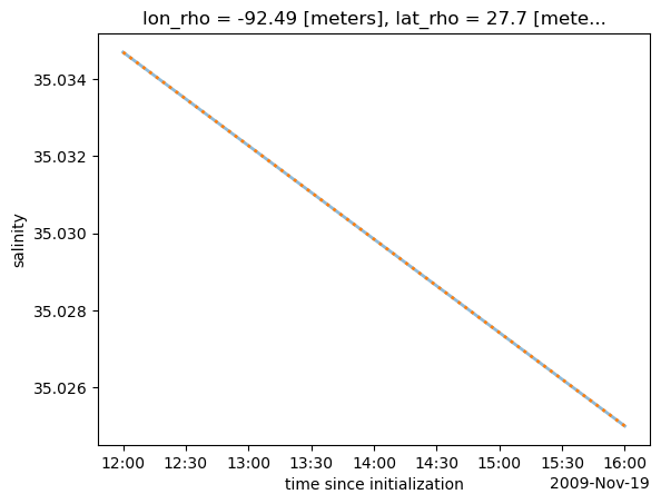
Here is an example of computing a rolling average in time. Nothing happens in this example because we only have two time steps to use, however, it does demonstrate the syntax. If more time steps were available we would update ds.salt.rolling(ocean_time=1) to include more time steps to average over in a rolling sense.
More information about rolling operations is available.
roll = ds.salt.rolling(ocean_time=1, center=True, min_periods=1).mean()
roll.isel(s_rho=-1, eta_rho=10, xi_rho=20).plot(alpha=0.5, lw=2)
ds.salt.isel(s_rho=-1, eta_rho=10, xi_rho=20).plot(ls=":", lw=2)
[<matplotlib.lines.Line2D at 0x758ebf6e3080>]
Resampling in time
Can’t have any chunks in the time dimension to do this. More info: http://xarray.pydata.org/en/stable/generated/xarray.Dataset.resample.html
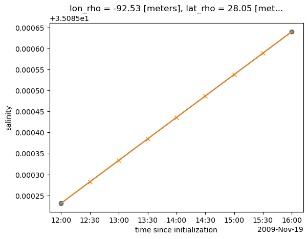
Upsample
Upsample to a higher resolution in time. Makes sense to interpolate to fill in data when upsampling, but can also forward or backfill, or just add nan’s.
dstest = ds.resample(ocean_time='30min', restore_coord_dims=True).interpolate()
Plot to visually inspect results
ds.salt.cf.isel(Y=30, X=20, Z=-1).plot(marker='o')
dstest.salt.cf.isel(Y=30, X=20, Z=-1).plot(marker='x')
[<matplotlib.lines.Line2D at 0x758ebe565940>]
Downsample
Resample down to lower resolution in time. This requires appending a method to aggregate the extra data, such as a mean. Note that other options can be used to shift the result within the interval of aggregation in various ways. Just the syntax is shown here since we only have two time steps to work with.
dstest = ds.resample(ocean_time='6H').mean()
ds.salt.cf.isel(Y=30, X=20, Z=-1).plot(marker='o')
dstest.salt.cf.isel(Y=30, X=20, Z=-1).plot(marker='x')
Seasonal average, over time
This is an example of resampling.
da.cf.resample({'T': [time frequency string]}).reduce([aggregation function])
For example, calculate the mean temperature every quarter in time with the following:
ds.temp.cf.resample({'T': 'QS'}).reduce(np.mean)
or the aggregation function can be appended on the end directly with:
ds.temp.cf.resample({'T': 'QS'}).mean()
The result of this calculation is a time series of downsampled chunks of output in time, the frequency of which is selected by input “time frequency string”, and aggregated by input “aggregation function”.
Examples of the time frequency string are:
“QS”: quarters, starting in January of each year and averaging three months.
Also available are selections like “QS-DEC”, quarters but starting with December to better align with seasons. Other months are input options as well.
“MS”: monthly
“D”: daily
“H”: hourly
Many more options are given here.
Examples of aggregation functions are:
np.mean
np.max
np.min
np.sum
np.std
Result of downsampling a 4D salt array from hourly to 6-hourly, for example, gives: [ocean_time x s_rho x eta_rho x xi_rho], where ocean_time has about 1/6 of the number of entries reflecting the aggregation in time.
ds.temp.cf.resample(indexer={'T': '6H'}).reduce(np.mean)
/home/docs/checkouts/readthedocs.org/user_builds/xroms/conda/stable/lib/python3.12/site-packages/xarray/groupers.py:509: FutureWarning: 'H' is deprecated and will be removed in a future version, please use 'h' instead.
  self.index_grouper = pd.Grouper(
<xarray.DataArray 'temp' (ocean_time: 1, s_rho: 30, eta_rho: 191, xi_rho: 300)> Size: 7MB
dask.array<stack, shape=(1, 30, 191, 300), dtype=float32, chunksize=(1, 30, 191, 300), chunktype=numpy.ndarray>
Coordinates:
    lon_rho     (eta_rho, xi_rho) float64 458kB dask.array<chunksize=(191, 300), meta=np.ndarray>
    lat_rho     (eta_rho, xi_rho) float64 458kB dask.array<chunksize=(191, 300), meta=np.ndarray>
  * s_rho       (s_rho) float64 240B -0.9833 -0.95 -0.9167 ... -0.05 -0.01667
  * xi_rho      (xi_rho) int64 2kB 0 1 2 3 4 5 6 ... 293 294 295 296 297 298 299
  * eta_rho     (eta_rho) int64 2kB 0 1 2 3 4 5 6 ... 185 186 187 188 189 190
  * ocean_time  (ocean_time) datetime64[ns] 8B 2009-11-19T12:00:00
Attributes:
    long_name:  potential temperature
    units:      Celsius
    time:       ocean_time
field: temperature, scalar, seriesSeasonal mean over all available time
This is how to average over the full dataset period by certain time groupings using xarray groupby which is like pandas version. In this case we show the seasonal mean averaged across the full model time period. The syntax for this is:
da.salt.cf.groupby('T.[time string]').reduce([aggregation function])
For example, to average salt by season:
da.salt.cf.groupby('T.season').reduce(np.mean)
or
da.salt.cf.groupby('T.season').mean()
Options for the time string include:
‘season’
‘year’
‘month’
‘day’
‘hour’
‘minute’
‘second’
‘dayofyear’
‘week’
‘dayofweek’
‘weekday’
‘quarter’
More information about options for time (including “derived” datetime coordinates) is here.
Examples of aggregation functions are:
np.mean
np.max
np.min
np.sum
np.std
Result of averaging over seasons for a 4D salt array returns, for example: [season x s_rho x eta_rho x xi_rho], where season has 4 entries, each covering 3 months of the year.
# this example has only 1 season because it is a short example file
ds.temp.cf.groupby('T.season').mean()
<xarray.DataArray 'temp' (season: 1, s_rho: 30, eta_rho: 191, xi_rho: 300)> Size: 7MB
dask.array<stack, shape=(1, 30, 191, 300), dtype=float32, chunksize=(1, 30, 191, 300), chunktype=numpy.ndarray>
Coordinates:
lon_rho (eta_rho, xi_rho) float64 458kB dask.array<chunksize=(191, 300), meta=np.ndarray>
lat_rho (eta_rho, xi_rho) float64 458kB dask.array<chunksize=(191, 300), meta=np.ndarray>
* s_rho (s_rho) float64 240B -0.9833 -0.95 -0.9167 ... -0.05 -0.01667
* xi_rho (xi_rho) int64 2kB 0 1 2 3 4 5 6 7 ... 293 294 295 296 297 298 299
* eta_rho (eta_rho) int64 2kB 0 1 2 3 4 5 6 7 ... 184 185 186 187 188 189 190
* season (season) object 8B 'SON'
Attributes:
long_name: potential temperature
units: Celsius
time: ocean_time
field: temperature, scalar, series