import xarray as xr
import xroms
import numpy as np
import matplotlib.pyplot as plt
import cmocean.cm as cmo
import pandas as pd
How to interpolate
There is a different approach for interpolation in:
time (using
xarray interp)longitude/latitude (using
xESMF)depth (using
xgcm)
In this notebook, we will demonstrate each independently as well considerations for combining the approaches.
Load in data
Load in example dataset. More information at in input/output page
ds = xroms.datasets.fetch_ROMS_example_full_grid()
ds, xgrid = xroms.roms_dataset(ds, include_cell_volume=True, include_Z0=True)
ds.xroms.set_grid(xgrid)
ds
<xarray.Dataset> Size: 957MB
Dimensions: (eta_rho: 191, xi_rho: 300, s_rho: 30, ocean_time: 2, s_w: 31,
xi_u: 299, eta_v: 190)
Coordinates: (12/29)
lon_rho (eta_rho, xi_rho) float64 458kB dask.array<chunksize=(191, 300), meta=np.ndarray>
lat_rho (eta_rho, xi_rho) float64 458kB dask.array<chunksize=(191, 300), meta=np.ndarray>
* s_rho (s_rho) float64 240B -0.9833 -0.95 -0.9167 ... -0.05 -0.01667
* s_w (s_w) float64 248B -1.0 -0.9667 -0.9333 ... -0.03333 0.0
* ocean_time (ocean_time) datetime64[ns] 16B 2009-11-19T12:00:00 2009-11-1...
lon_u (eta_rho, xi_u) float64 457kB dask.array<chunksize=(191, 299), meta=np.ndarray>
... ...
z_rho_v0 (s_rho, eta_v, xi_rho) float64 14MB dask.array<chunksize=(30, 190, 300), meta=np.ndarray>
z_rho_psi0 (s_rho, eta_v, xi_u) float64 14MB dask.array<chunksize=(30, 190, 299), meta=np.ndarray>
z_w0 (s_w, eta_rho, xi_rho) float64 14MB dask.array<chunksize=(31, 191, 300), meta=np.ndarray>
z_w_u0 (s_w, eta_rho, xi_u) float64 14MB dask.array<chunksize=(31, 191, 299), meta=np.ndarray>
z_w_v0 (s_w, eta_v, xi_rho) float64 14MB dask.array<chunksize=(31, 190, 300), meta=np.ndarray>
z_w_psi0 (s_w, eta_v, xi_u) float64 14MB dask.array<chunksize=(31, 190, 299), meta=np.ndarray>
Data variables: (12/53)
angle (eta_rho, xi_rho) float64 458kB dask.array<chunksize=(191, 300), meta=np.ndarray>
hc float64 8B ...
Cs_r (s_rho) float64 240B dask.array<chunksize=(30,), meta=np.ndarray>
zeta (ocean_time, eta_rho, xi_rho) float32 458kB dask.array<chunksize=(2, 191, 300), meta=np.ndarray>
h (eta_rho, xi_rho) float64 458kB dask.array<chunksize=(191, 300), meta=np.ndarray>
Cs_w (s_w) float64 248B dask.array<chunksize=(31,), meta=np.ndarray>
... ...
dV_w_u (ocean_time, s_w, eta_rho, xi_u) float64 28MB dask.array<chunksize=(2, 31, 191, 299), meta=np.ndarray>
dV_v (ocean_time, s_rho, eta_v, xi_rho) float64 27MB dask.array<chunksize=(2, 30, 190, 300), meta=np.ndarray>
dV_w_v (ocean_time, s_w, eta_v, xi_rho) float64 28MB dask.array<chunksize=(2, 31, 190, 300), meta=np.ndarray>
dV_psi (ocean_time, s_rho, eta_v, xi_u) float64 27MB dask.array<chunksize=(2, 30, 190, 299), meta=np.ndarray>
dV_w_psi (ocean_time, s_w, eta_v, xi_u) float64 28MB dask.array<chunksize=(2, 31, 190, 299), meta=np.ndarray>
rho0 int64 8B 1025
Attributes: (12/29)
file: ocean_his_0150.nc
format: netCDF-3 classic file
Conventions: CF-1.4
type: ROMS/TOMS history file
title: Texas and Louisiana Shelf case (Nesting)
rst_file: ocean_rst.nc
... ...
compiler_command: /g/software/openmpi/1.4.3/intel/bin/mpif90
compiler_flags: -heap-arrays -fp-model precise -assume 2underscores -c...
tiling: 016x032
history: ROMS/TOMS, Version 3.4, Sunday - December 4, 2011 - 7...
ana_file: /scratch/zhangxq/projects/txla_nesting6/Functionals/an...
CPP_options: TXLA, ANA_BSFLUX, ANA_BTFLUX, ASSUMED_SHAPE, BULK_FLUX...- eta_rho: 191
- xi_rho: 300
- s_rho: 30
- ocean_time: 2
- s_w: 31
- xi_u: 299
- eta_v: 190
- lon_rho(eta_rho, xi_rho)float64dask.array<chunksize=(191, 300), meta=np.ndarray>
- units :
- meters
- standard_name :
- longitude
Array Chunk Bytes 447.66 kiB 447.66 kiB Shape (191, 300) (191, 300) Dask graph 1 chunks in 2 graph layers Data type float64 numpy.ndarray 300 191 - lat_rho(eta_rho, xi_rho)float64dask.array<chunksize=(191, 300), meta=np.ndarray>
- units :
- meters
- standard_name :
- latitude
Array Chunk Bytes 447.66 kiB 447.66 kiB Shape (191, 300) (191, 300) Dask graph 1 chunks in 2 graph layers Data type float64 numpy.ndarray 300 191 - s_rho(s_rho)float64-0.9833 -0.95 ... -0.05 -0.01667
- long_name :
- S-coordinate at RHO-points
- valid_min :
- -1.0
- valid_max :
- 0.0
- standard_name :
- ocean_s_coordinate_g1
- formula_terms :
- s: s_rho C: Cs_r eta: zeta depth: h depth_c: hc
- field :
- s_rho, scalar
- axis :
- Z
array([-0.983333, -0.95 , -0.916667, -0.883333, -0.85 , -0.816667, -0.783333, -0.75 , -0.716667, -0.683333, -0.65 , -0.616667, -0.583333, -0.55 , -0.516667, -0.483333, -0.45 , -0.416667, -0.383333, -0.35 , -0.316667, -0.283333, -0.25 , -0.216667, -0.183333, -0.15 , -0.116667, -0.083333, -0.05 , -0.016667]) - s_w(s_w)float64-1.0 -0.9667 ... -0.03333 0.0
- long_name :
- S-coordinate at W-points
- valid_min :
- -1.0
- valid_max :
- 0.0
- standard_name :
- ocean_s_coordinate_g1
- formula_terms :
- s: s_w C: Cs_w eta: zeta depth: h depth_c: hc
- field :
- s_w, scalar
- axis :
- Z
array([-1. , -0.966667, -0.933333, -0.9 , -0.866667, -0.833333, -0.8 , -0.766667, -0.733333, -0.7 , -0.666667, -0.633333, -0.6 , -0.566667, -0.533333, -0.5 , -0.466667, -0.433333, -0.4 , -0.366667, -0.333333, -0.3 , -0.266667, -0.233333, -0.2 , -0.166667, -0.133333, -0.1 , -0.066667, -0.033333, 0. ]) - ocean_time(ocean_time)datetime64[ns]2009-11-19T12:00:00 2009-11-19T1...
- long_name :
- time since initialization
- field :
- time, scalar, series
- axis :
- T
- standard_name :
- time
array(['2009-11-19T12:00:00.000000000', '2009-11-19T16:00:00.000000000'], dtype='datetime64[ns]') - lon_u(eta_rho, xi_u)float64dask.array<chunksize=(191, 299), meta=np.ndarray>
- units :
- meters
- standard_name :
- longitude
Array Chunk Bytes 446.16 kiB 446.16 kiB Shape (191, 299) (191, 299) Dask graph 1 chunks in 2 graph layers Data type float64 numpy.ndarray 299 191 - lat_u(eta_rho, xi_u)float64dask.array<chunksize=(191, 299), meta=np.ndarray>
- units :
- meters
- standard_name :
- latitude
Array Chunk Bytes 446.16 kiB 446.16 kiB Shape (191, 299) (191, 299) Dask graph 1 chunks in 2 graph layers Data type float64 numpy.ndarray 299 191 - lon_v(eta_v, xi_rho)float64dask.array<chunksize=(190, 300), meta=np.ndarray>
- units :
- meters
- standard_name :
- longitude
Array Chunk Bytes 445.31 kiB 445.31 kiB Shape (190, 300) (190, 300) Dask graph 1 chunks in 2 graph layers Data type float64 numpy.ndarray 300 190 - lat_v(eta_v, xi_rho)float64dask.array<chunksize=(190, 300), meta=np.ndarray>
- units :
- meters
- standard_name :
- latitude
Array Chunk Bytes 445.31 kiB 445.31 kiB Shape (190, 300) (190, 300) Dask graph 1 chunks in 2 graph layers Data type float64 numpy.ndarray 300 190 - xi_rho(xi_rho)int640 1 2 3 4 5 ... 295 296 297 298 299
- axis :
- X
array([ 0, 1, 2, ..., 297, 298, 299], shape=(300,))
- xi_u(xi_u)int640 1 2 3 4 5 ... 294 295 296 297 298
- axis :
- X
array([ 0, 1, 2, ..., 296, 297, 298], shape=(299,))
- eta_rho(eta_rho)int640 1 2 3 4 5 ... 186 187 188 189 190
- axis :
- Y
array([ 0, 1, 2, 3, 4, 5, 6, 7, 8, 9, 10, 11, 12, 13, 14, 15, 16, 17, 18, 19, 20, 21, 22, 23, 24, 25, 26, 27, 28, 29, 30, 31, 32, 33, 34, 35, 36, 37, 38, 39, 40, 41, 42, 43, 44, 45, 46, 47, 48, 49, 50, 51, 52, 53, 54, 55, 56, 57, 58, 59, 60, 61, 62, 63, 64, 65, 66, 67, 68, 69, 70, 71, 72, 73, 74, 75, 76, 77, 78, 79, 80, 81, 82, 83, 84, 85, 86, 87, 88, 89, 90, 91, 92, 93, 94, 95, 96, 97, 98, 99, 100, 101, 102, 103, 104, 105, 106, 107, 108, 109, 110, 111, 112, 113, 114, 115, 116, 117, 118, 119, 120, 121, 122, 123, 124, 125, 126, 127, 128, 129, 130, 131, 132, 133, 134, 135, 136, 137, 138, 139, 140, 141, 142, 143, 144, 145, 146, 147, 148, 149, 150, 151, 152, 153, 154, 155, 156, 157, 158, 159, 160, 161, 162, 163, 164, 165, 166, 167, 168, 169, 170, 171, 172, 173, 174, 175, 176, 177, 178, 179, 180, 181, 182, 183, 184, 185, 186, 187, 188, 189, 190]) - eta_v(eta_v)int640 1 2 3 4 5 ... 185 186 187 188 189
- axis :
- Y
array([ 0, 1, 2, 3, 4, 5, 6, 7, 8, 9, 10, 11, 12, 13, 14, 15, 16, 17, 18, 19, 20, 21, 22, 23, 24, 25, 26, 27, 28, 29, 30, 31, 32, 33, 34, 35, 36, 37, 38, 39, 40, 41, 42, 43, 44, 45, 46, 47, 48, 49, 50, 51, 52, 53, 54, 55, 56, 57, 58, 59, 60, 61, 62, 63, 64, 65, 66, 67, 68, 69, 70, 71, 72, 73, 74, 75, 76, 77, 78, 79, 80, 81, 82, 83, 84, 85, 86, 87, 88, 89, 90, 91, 92, 93, 94, 95, 96, 97, 98, 99, 100, 101, 102, 103, 104, 105, 106, 107, 108, 109, 110, 111, 112, 113, 114, 115, 116, 117, 118, 119, 120, 121, 122, 123, 124, 125, 126, 127, 128, 129, 130, 131, 132, 133, 134, 135, 136, 137, 138, 139, 140, 141, 142, 143, 144, 145, 146, 147, 148, 149, 150, 151, 152, 153, 154, 155, 156, 157, 158, 159, 160, 161, 162, 163, 164, 165, 166, 167, 168, 169, 170, 171, 172, 173, 174, 175, 176, 177, 178, 179, 180, 181, 182, 183, 184, 185, 186, 187, 188, 189]) - z_w(ocean_time, s_w, eta_rho, xi_rho)float64dask.array<chunksize=(2, 31, 191, 300), meta=np.ndarray>
- long_name :
- depth of W-points
- time :
- ocean_time
- field :
- z_w, scalar, series
- units :
- m
- positive :
- up
- standard_name :
- depth
Array Chunk Bytes 27.10 MiB 27.10 MiB Shape (2, 31, 191, 300) (2, 31, 191, 300) Dask graph 1 chunks in 29 graph layers Data type float64 numpy.ndarray 2 1 300 191 31 - z_w_u(ocean_time, s_w, eta_rho, xi_u)float64dask.array<chunksize=(2, 31, 191, 299), meta=np.ndarray>
- long_name :
- depth of U-points on vertical W grid
- time :
- ocean_time
- field :
- z_w_u, scalar, series
- units :
- m
- positive :
- up
- standard_name :
- depth
Array Chunk Bytes 27.01 MiB 27.01 MiB Shape (2, 31, 191, 299) (2, 31, 191, 299) Dask graph 1 chunks in 32 graph layers Data type float64 numpy.ndarray 2 1 299 191 31 - z_w_v(ocean_time, s_w, eta_v, xi_rho)float64dask.array<chunksize=(2, 31, 190, 300), meta=np.ndarray>
- long_name :
- depth of V-points on vertical W grid
- time :
- ocean_time
- field :
- z_w_v, scalar, series
- units :
- m
- positive :
- up
- standard_name :
- depth
Array Chunk Bytes 26.96 MiB 26.96 MiB Shape (2, 31, 190, 300) (2, 31, 190, 300) Dask graph 1 chunks in 34 graph layers Data type float64 numpy.ndarray 2 1 300 190 31 - z_w_psi(ocean_time, s_w, eta_v, xi_u)float64dask.array<chunksize=(2, 31, 190, 299), meta=np.ndarray>
- long_name :
- depth of PSI-points on vertical W grid
- time :
- ocean_time
- field :
- z_w_psi, scalar, series
- units :
- m
- positive :
- up
- standard_name :
- depth
Array Chunk Bytes 26.87 MiB 26.87 MiB Shape (2, 31, 190, 299) (2, 31, 190, 299) Dask graph 1 chunks in 37 graph layers Data type float64 numpy.ndarray 2 1 299 190 31 - z_rho(ocean_time, s_rho, eta_rho, xi_rho)float64dask.array<chunksize=(2, 30, 191, 300), meta=np.ndarray>
- long_name :
- depth of RHO-points
- time :
- ocean_time
- field :
- z_rho, scalar, series
- units :
- m
- positive :
- up
- standard_name :
- depth
Array Chunk Bytes 26.23 MiB 26.23 MiB Shape (2, 30, 191, 300) (2, 30, 191, 300) Dask graph 1 chunks in 29 graph layers Data type float64 numpy.ndarray 2 1 300 191 30 - z_rho_u(ocean_time, s_rho, eta_rho, xi_u)float64dask.array<chunksize=(2, 30, 191, 299), meta=np.ndarray>
- long_name :
- depth of U-points on vertical RHO grid
- time :
- ocean_time
- field :
- z_rho_u, scalar, series
- units :
- m
- positive :
- up
- standard_name :
- depth
Array Chunk Bytes 26.14 MiB 26.14 MiB Shape (2, 30, 191, 299) (2, 30, 191, 299) Dask graph 1 chunks in 32 graph layers Data type float64 numpy.ndarray 2 1 299 191 30 - z_rho_v(ocean_time, s_rho, eta_v, xi_rho)float64dask.array<chunksize=(2, 30, 190, 300), meta=np.ndarray>
- long_name :
- depth of V-points on vertical RHO grid
- time :
- ocean_time
- field :
- z_rho_v, scalar, series
- units :
- m
- positive :
- up
- standard_name :
- depth
Array Chunk Bytes 26.09 MiB 26.09 MiB Shape (2, 30, 190, 300) (2, 30, 190, 300) Dask graph 1 chunks in 34 graph layers Data type float64 numpy.ndarray 2 1 300 190 30 - z_rho_psi(ocean_time, s_rho, eta_v, xi_u)float64dask.array<chunksize=(2, 30, 190, 299), meta=np.ndarray>
- long_name :
- depth of PSI-points on vertical RHO grid
- time :
- ocean_time
- field :
- z_rho_psi, scalar, series
- units :
- m
- positive :
- up
- standard_name :
- depth
Array Chunk Bytes 26.01 MiB 26.01 MiB Shape (2, 30, 190, 299) (2, 30, 190, 299) Dask graph 1 chunks in 37 graph layers Data type float64 numpy.ndarray 2 1 299 190 30 - z_rho0(s_rho, eta_rho, xi_rho)float64dask.array<chunksize=(30, 191, 300), meta=np.ndarray>
- long_name :
- depth of RHO-points
- field :
- z_rho0, scalar
- units :
- m
Array Chunk Bytes 13.11 MiB 13.11 MiB Shape (30, 191, 300) (30, 191, 300) Dask graph 1 chunks in 15 graph layers Data type float64 numpy.ndarray 300 191 30 - z_rho_u0(s_rho, eta_rho, xi_u)float64dask.array<chunksize=(30, 191, 299), meta=np.ndarray>
- long_name :
- depth of U-points on vertical RHO grid
- field :
- z_rho_u0, scalar
- units :
- m
Array Chunk Bytes 13.07 MiB 13.07 MiB Shape (30, 191, 299) (30, 191, 299) Dask graph 1 chunks in 18 graph layers Data type float64 numpy.ndarray 299 191 30 - z_rho_v0(s_rho, eta_v, xi_rho)float64dask.array<chunksize=(30, 190, 300), meta=np.ndarray>
- long_name :
- depth of V-points on vertical RHO grid
- field :
- z_rho_v0, scalar
- units :
- m
Array Chunk Bytes 13.05 MiB 13.05 MiB Shape (30, 190, 300) (30, 190, 300) Dask graph 1 chunks in 20 graph layers Data type float64 numpy.ndarray 300 190 30 - z_rho_psi0(s_rho, eta_v, xi_u)float64dask.array<chunksize=(30, 190, 299), meta=np.ndarray>
- long_name :
- depth of PSI-points on vertical RHO grid
- field :
- z_rho_psi0, scalar
- units :
- m
Array Chunk Bytes 13.00 MiB 13.00 MiB Shape (30, 190, 299) (30, 190, 299) Dask graph 1 chunks in 23 graph layers Data type float64 numpy.ndarray 299 190 30 - z_w0(s_w, eta_rho, xi_rho)float64dask.array<chunksize=(31, 191, 300), meta=np.ndarray>
- long_name :
- depth of W-points
- field :
- z_w0, scalar
- units :
- m
Array Chunk Bytes 13.55 MiB 13.55 MiB Shape (31, 191, 300) (31, 191, 300) Dask graph 1 chunks in 15 graph layers Data type float64 numpy.ndarray 300 191 31 - z_w_u0(s_w, eta_rho, xi_u)float64dask.array<chunksize=(31, 191, 299), meta=np.ndarray>
- long_name :
- depth of U-points on vertical W grid
- field :
- z_w_u0, scalar
- units :
- m
Array Chunk Bytes 13.51 MiB 13.51 MiB Shape (31, 191, 299) (31, 191, 299) Dask graph 1 chunks in 18 graph layers Data type float64 numpy.ndarray 299 191 31 - z_w_v0(s_w, eta_v, xi_rho)float64dask.array<chunksize=(31, 190, 300), meta=np.ndarray>
- long_name :
- depth of V-points on vertical W grid
- field :
- z_w_v0, scalar
- units :
- m
Array Chunk Bytes 13.48 MiB 13.48 MiB Shape (31, 190, 300) (31, 190, 300) Dask graph 1 chunks in 20 graph layers Data type float64 numpy.ndarray 300 190 31 - z_w_psi0(s_w, eta_v, xi_u)float64dask.array<chunksize=(31, 190, 299), meta=np.ndarray>
- long_name :
- depth of PSI-points on vertical W grid
- field :
- z_w_psi0, scalar
- units :
- m
Array Chunk Bytes 13.44 MiB 13.44 MiB Shape (31, 190, 299) (31, 190, 299) Dask graph 1 chunks in 23 graph layers Data type float64 numpy.ndarray 299 190 31
- angle(eta_rho, xi_rho)float64dask.array<chunksize=(191, 300), meta=np.ndarray>
- long_name :
- angle between XI-axis and EAST
- units :
- radians
- field :
- angle, scalar
Array Chunk Bytes 447.66 kiB 447.66 kiB Shape (191, 300) (191, 300) Dask graph 1 chunks in 2 graph layers Data type float64 numpy.ndarray 300 191 - hc()float64...
- long_name :
- S-coordinate parameter, critical depth
- units :
- meter
[1 values with dtype=float64]
- Cs_r(s_rho)float64dask.array<chunksize=(30,), meta=np.ndarray>
- long_name :
- S-coordinate stretching curves at RHO-points
- valid_min :
- -1.0
- valid_max :
- 0.0
- field :
- Cs_r, scalar
Array Chunk Bytes 240 B 240 B Shape (30,) (30,) Dask graph 1 chunks in 2 graph layers Data type float64 numpy.ndarray 30 1 - zeta(ocean_time, eta_rho, xi_rho)float32dask.array<chunksize=(2, 191, 300), meta=np.ndarray>
- long_name :
- free-surface
- units :
- meter
- time :
- ocean_time
- field :
- free-surface, scalar, series
Array Chunk Bytes 447.66 kiB 447.66 kiB Shape (2, 191, 300) (2, 191, 300) Dask graph 1 chunks in 2 graph layers Data type float32 numpy.ndarray 300 191 2 - h(eta_rho, xi_rho)float64dask.array<chunksize=(191, 300), meta=np.ndarray>
- long_name :
- bathymetry at RHO-points
- units :
- meter
- field :
- bath, scalar
Array Chunk Bytes 447.66 kiB 447.66 kiB Shape (191, 300) (191, 300) Dask graph 1 chunks in 2 graph layers Data type float64 numpy.ndarray 300 191 - Cs_w(s_w)float64dask.array<chunksize=(31,), meta=np.ndarray>
- long_name :
- S-coordinate stretching curves at W-points
- valid_min :
- -1.0
- valid_max :
- 0.0
- field :
- Cs_w, scalar
Array Chunk Bytes 248 B 248 B Shape (31,) (31,) Dask graph 1 chunks in 2 graph layers Data type float64 numpy.ndarray 31 1 - mask_rho(eta_rho, xi_rho)float64dask.array<chunksize=(191, 300), meta=np.ndarray>
- long_name :
- mask on RHO-points
- flag_values :
- [0. 1.]
- flag_meanings :
- land water
Array Chunk Bytes 447.66 kiB 447.66 kiB Shape (191, 300) (191, 300) Dask graph 1 chunks in 2 graph layers Data type float64 numpy.ndarray 300 191 - mask_u(eta_rho, xi_u)float64dask.array<chunksize=(191, 299), meta=np.ndarray>
- long_name :
- mask on U-points
- flag_values :
- [0. 1.]
- flag_meanings :
- land water
Array Chunk Bytes 446.16 kiB 446.16 kiB Shape (191, 299) (191, 299) Dask graph 1 chunks in 2 graph layers Data type float64 numpy.ndarray 299 191 - mask_v(eta_v, xi_rho)float64dask.array<chunksize=(190, 300), meta=np.ndarray>
- long_name :
- mask on V-points
- flag_values :
- [0. 1.]
- flag_meanings :
- land water
Array Chunk Bytes 445.31 kiB 445.31 kiB Shape (190, 300) (190, 300) Dask graph 1 chunks in 2 graph layers Data type float64 numpy.ndarray 300 190 - u(ocean_time, s_rho, eta_rho, xi_u)float32dask.array<chunksize=(2, 30, 191, 299), meta=np.ndarray>
- long_name :
- u-momentum component
- units :
- meter second-1
- time :
- ocean_time
- field :
- u-velocity, scalar, series
Array Chunk Bytes 13.07 MiB 13.07 MiB Shape (2, 30, 191, 299) (2, 30, 191, 299) Dask graph 1 chunks in 2 graph layers Data type float32 numpy.ndarray 2 1 299 191 30 - v(ocean_time, s_rho, eta_v, xi_rho)float32dask.array<chunksize=(2, 30, 190, 300), meta=np.ndarray>
- long_name :
- v-momentum component
- units :
- meter second-1
- time :
- ocean_time
- field :
- v-velocity, scalar, series
Array Chunk Bytes 13.05 MiB 13.05 MiB Shape (2, 30, 190, 300) (2, 30, 190, 300) Dask graph 1 chunks in 2 graph layers Data type float32 numpy.ndarray 2 1 300 190 30 - temp(ocean_time, s_rho, eta_rho, xi_rho)float32dask.array<chunksize=(2, 30, 191, 300), meta=np.ndarray>
- long_name :
- potential temperature
- units :
- Celsius
- time :
- ocean_time
- field :
- temperature, scalar, series
Array Chunk Bytes 13.11 MiB 13.11 MiB Shape (2, 30, 191, 300) (2, 30, 191, 300) Dask graph 1 chunks in 2 graph layers Data type float32 numpy.ndarray 2 1 300 191 30 - salt(ocean_time, s_rho, eta_rho, xi_rho)float32dask.array<chunksize=(2, 30, 191, 300), meta=np.ndarray>
- long_name :
- salinity
- time :
- ocean_time
- field :
- salinity, scalar, series
Array Chunk Bytes 13.11 MiB 13.11 MiB Shape (2, 30, 191, 300) (2, 30, 191, 300) Dask graph 1 chunks in 2 graph layers Data type float32 numpy.ndarray 2 1 300 191 30 - Vtransform()int32...
- long_name :
- vertical terrain-following transformation equation
[1 values with dtype=int32]
- pm(eta_rho, xi_rho)float64dask.array<chunksize=(191, 300), meta=np.ndarray>
- long_name :
- curvilinear coordinate metric in XI
- units :
- meter-1
- field :
- pm, scalar
Array Chunk Bytes 447.66 kiB 447.66 kiB Shape (191, 300) (191, 300) Dask graph 1 chunks in 2 graph layers Data type float64 numpy.ndarray 300 191 - pn(eta_rho, xi_rho)float64dask.array<chunksize=(191, 300), meta=np.ndarray>
- long_name :
- curvilinear coordinate metric in ETA
- units :
- meter-1
- field :
- pn, scalar
Array Chunk Bytes 447.66 kiB 447.66 kiB Shape (191, 300) (191, 300) Dask graph 1 chunks in 2 graph layers Data type float64 numpy.ndarray 300 191 - f(eta_rho, xi_rho)float64dask.array<chunksize=(191, 300), meta=np.ndarray>
- long_name :
- Coriolis parameter at RHO-points
- units :
- second-1
- field :
- coriolis, scalar
Array Chunk Bytes 447.66 kiB 447.66 kiB Shape (191, 300) (191, 300) Dask graph 1 chunks in 2 graph layers Data type float64 numpy.ndarray 300 191 - spherical()int641
array(1)
- 3d()boolTrue
array(True)
- dx(eta_rho, xi_rho)float64dask.array<chunksize=(191, 300), meta=np.ndarray>
- long_name :
- inverse curvilinear coordinate metric in XI
- units :
- meter
- field :
- dx, scalar
Array Chunk Bytes 447.66 kiB 447.66 kiB Shape (191, 300) (191, 300) Dask graph 1 chunks in 3 graph layers Data type float64 numpy.ndarray 300 191 - dx_u(eta_rho, xi_u)float64dask.array<chunksize=(191, 299), meta=np.ndarray>
- long_name :
- inverse curvilinear coordinate metric in XI on U grid
- units :
- meter
- field :
- dx_u, scalar
Array Chunk Bytes 446.16 kiB 446.16 kiB Shape (191, 299) (191, 299) Dask graph 1 chunks in 6 graph layers Data type float64 numpy.ndarray 299 191 - dx_v(eta_v, xi_rho)float64dask.array<chunksize=(190, 300), meta=np.ndarray>
- long_name :
- inverse curvilinear coordinate metric in XI on V grid
- units :
- meter
- field :
- dx_v, scalar
Array Chunk Bytes 445.31 kiB 445.31 kiB Shape (190, 300) (190, 300) Dask graph 1 chunks in 8 graph layers Data type float64 numpy.ndarray 300 190 - dx_psi(eta_v, xi_u)float64dask.array<chunksize=(190, 299), meta=np.ndarray>
- long_name :
- inverse curvilinear coordinate metric in XI on PSI grid
- units :
- meter
- field :
- dx_psi, scalar
Array Chunk Bytes 443.83 kiB 443.83 kiB Shape (190, 299) (190, 299) Dask graph 1 chunks in 11 graph layers Data type float64 numpy.ndarray 299 190 - dy(eta_rho, xi_rho)float64dask.array<chunksize=(191, 300), meta=np.ndarray>
- long_name :
- inverse curvilinear coordinate metric in ETA
- units :
- meter
- field :
- dy, scalar
Array Chunk Bytes 447.66 kiB 447.66 kiB Shape (191, 300) (191, 300) Dask graph 1 chunks in 3 graph layers Data type float64 numpy.ndarray 300 191 - dy_u(eta_rho, xi_u)float64dask.array<chunksize=(191, 299), meta=np.ndarray>
- long_name :
- inverse curvilinear coordinate metric in ETA on U grid
- units :
- meter
- field :
- dy_u, scalar
Array Chunk Bytes 446.16 kiB 446.16 kiB Shape (191, 299) (191, 299) Dask graph 1 chunks in 6 graph layers Data type float64 numpy.ndarray 299 191 - dy_v(eta_v, xi_rho)float64dask.array<chunksize=(190, 300), meta=np.ndarray>
- long_name :
- inverse curvilinear coordinate metric in ETA on V grid
- units :
- meter
- field :
- dy_v, scalar
Array Chunk Bytes 445.31 kiB 445.31 kiB Shape (190, 300) (190, 300) Dask graph 1 chunks in 8 graph layers Data type float64 numpy.ndarray 300 190 - dy_psi(eta_v, xi_u)float64dask.array<chunksize=(190, 299), meta=np.ndarray>
- long_name :
- inverse curvilinear coordinate metric in ETA on PSI grid
- units :
- meter
- field :
- dy_psi, scalar
Array Chunk Bytes 443.83 kiB 443.83 kiB Shape (190, 299) (190, 299) Dask graph 1 chunks in 11 graph layers Data type float64 numpy.ndarray 299 190 - dz(ocean_time, s_rho, eta_rho, xi_rho)float64dask.array<chunksize=(2, 30, 191, 300), meta=np.ndarray>
- long_name :
- vertical layer thickness on vertical RHO grid
- time :
- ocean_time
- field :
- dz, scalar, series
- units :
- m
Array Chunk Bytes 26.23 MiB 26.23 MiB Shape (2, 30, 191, 300) (2, 30, 191, 300) Dask graph 1 chunks in 34 graph layers Data type float64 numpy.ndarray 2 1 300 191 30 - dz_w(ocean_time, s_w, eta_rho, xi_rho)float64dask.array<chunksize=(2, 31, 191, 300), meta=np.ndarray>
- long_name :
- vertical layer thickness on vertical W grid
- time :
- ocean_time
- field :
- dz_w, scalar, series
- units :
- m
Array Chunk Bytes 27.10 MiB 27.10 MiB Shape (2, 31, 191, 300) (2, 31, 191, 300) Dask graph 1 chunks in 38 graph layers Data type float64 numpy.ndarray 2 1 300 191 31 - dz_u(ocean_time, s_rho, eta_rho, xi_u)float64dask.array<chunksize=(2, 30, 191, 299), meta=np.ndarray>
- long_name :
- vertical layer thickness on vertical RHO grid on U grid
- time :
- ocean_time
- field :
- dz_u, scalar, series
- units :
- m
Array Chunk Bytes 26.14 MiB 26.14 MiB Shape (2, 30, 191, 299) (2, 30, 191, 299) Dask graph 1 chunks in 37 graph layers Data type float64 numpy.ndarray 2 1 299 191 30 - dz_w_u(ocean_time, s_w, eta_rho, xi_u)float64dask.array<chunksize=(2, 31, 191, 299), meta=np.ndarray>
- long_name :
- vertical layer thickness on vertical W grid on U grid
- time :
- ocean_time
- field :
- dz_w_u, scalar, series
- units :
- m
Array Chunk Bytes 27.01 MiB 27.01 MiB Shape (2, 31, 191, 299) (2, 31, 191, 299) Dask graph 1 chunks in 41 graph layers Data type float64 numpy.ndarray 2 1 299 191 31 - dz_v(ocean_time, s_rho, eta_v, xi_rho)float64dask.array<chunksize=(2, 30, 190, 300), meta=np.ndarray>
- long_name :
- vertical layer thickness on vertical RHO grid on V grid
- time :
- ocean_time
- field :
- dz_v, scalar, series
- units :
- m
Array Chunk Bytes 26.09 MiB 26.09 MiB Shape (2, 30, 190, 300) (2, 30, 190, 300) Dask graph 1 chunks in 39 graph layers Data type float64 numpy.ndarray 2 1 300 190 30 - dz_w_v(ocean_time, s_w, eta_v, xi_rho)float64dask.array<chunksize=(2, 31, 190, 300), meta=np.ndarray>
- long_name :
- vertical layer thickness on vertical W grid on V grid
- time :
- ocean_time
- field :
- dz_w_v, scalar, series
- units :
- m
Array Chunk Bytes 26.96 MiB 26.96 MiB Shape (2, 31, 190, 300) (2, 31, 190, 300) Dask graph 1 chunks in 43 graph layers Data type float64 numpy.ndarray 2 1 300 190 31 - dz_psi(ocean_time, s_rho, eta_v, xi_u)float64dask.array<chunksize=(2, 30, 190, 299), meta=np.ndarray>
- long_name :
- vertical layer thickness on vertical RHO grid on PSI grid
- time :
- ocean_time
- field :
- dz_psi, scalar, series
- units :
- m
Array Chunk Bytes 26.01 MiB 26.01 MiB Shape (2, 30, 190, 299) (2, 30, 190, 299) Dask graph 1 chunks in 42 graph layers Data type float64 numpy.ndarray 2 1 299 190 30 - dz_w_psi(ocean_time, s_w, eta_v, xi_u)float64dask.array<chunksize=(2, 31, 190, 299), meta=np.ndarray>
- long_name :
- vertical layer thickness on vertical W grid on PSI grid
- time :
- ocean_time
- field :
- dz_w_psi, scalar, series
- units :
- m
Array Chunk Bytes 26.87 MiB 26.87 MiB Shape (2, 31, 190, 299) (2, 31, 190, 299) Dask graph 1 chunks in 46 graph layers Data type float64 numpy.ndarray 2 1 299 190 31 - dz0(s_rho, eta_rho, xi_rho)float64dask.array<chunksize=(30, 191, 300), meta=np.ndarray>
- long_name :
- vertical layer thickness on vertical RHO grid
- field :
- dz0, scalar
- units :
- m
Array Chunk Bytes 13.11 MiB 13.11 MiB Shape (30, 191, 300) (30, 191, 300) Dask graph 1 chunks in 20 graph layers Data type float64 numpy.ndarray 300 191 30 - dz_w0(s_w, eta_rho, xi_rho)float64dask.array<chunksize=(31, 191, 300), meta=np.ndarray>
- long_name :
- vertical layer thickness on vertical W grid
- field :
- dz_w0, scalar
- units :
- m
Array Chunk Bytes 13.55 MiB 13.55 MiB Shape (31, 191, 300) (31, 191, 300) Dask graph 1 chunks in 24 graph layers Data type float64 numpy.ndarray 300 191 31 - dz_u0(s_rho, eta_rho, xi_u)float64dask.array<chunksize=(30, 191, 299), meta=np.ndarray>
- long_name :
- vertical layer thickness on vertical RHO grid on U grid
- field :
- dz_u0, scalar
- units :
- m
Array Chunk Bytes 13.07 MiB 13.07 MiB Shape (30, 191, 299) (30, 191, 299) Dask graph 1 chunks in 23 graph layers Data type float64 numpy.ndarray 299 191 30 - dz_w_u0(s_w, eta_rho, xi_u)float64dask.array<chunksize=(31, 191, 299), meta=np.ndarray>
- long_name :
- vertical layer thickness on vertical W grid on U grid
- field :
- dz_w_u0, scalar
- units :
- m
Array Chunk Bytes 13.51 MiB 13.51 MiB Shape (31, 191, 299) (31, 191, 299) Dask graph 1 chunks in 27 graph layers Data type float64 numpy.ndarray 299 191 31 - dz_v0(s_rho, eta_v, xi_rho)float64dask.array<chunksize=(30, 190, 300), meta=np.ndarray>
- long_name :
- vertical layer thickness on vertical RHO grid on V grid
- field :
- dz_v0, scalar
- units :
- m
Array Chunk Bytes 13.05 MiB 13.05 MiB Shape (30, 190, 300) (30, 190, 300) Dask graph 1 chunks in 25 graph layers Data type float64 numpy.ndarray 300 190 30 - dz_w_v0(s_w, eta_v, xi_rho)float64dask.array<chunksize=(31, 190, 300), meta=np.ndarray>
- long_name :
- vertical layer thickness on vertical W grid on V grid
- field :
- dz_w_v0, scalar
- units :
- m
Array Chunk Bytes 13.48 MiB 13.48 MiB Shape (31, 190, 300) (31, 190, 300) Dask graph 1 chunks in 29 graph layers Data type float64 numpy.ndarray 300 190 31 - dz_psi0(s_rho, eta_v, xi_u)float64dask.array<chunksize=(30, 190, 299), meta=np.ndarray>
- long_name :
- vertical layer thickness on vertical RHO grid on PSI grid
- field :
- dz_psi0, scalar
- units :
- m
Array Chunk Bytes 13.00 MiB 13.00 MiB Shape (30, 190, 299) (30, 190, 299) Dask graph 1 chunks in 28 graph layers Data type float64 numpy.ndarray 299 190 30 - dz_w_psi0(s_w, eta_v, xi_u)float64dask.array<chunksize=(31, 190, 299), meta=np.ndarray>
- long_name :
- vertical layer thickness on vertical W grid on PSI grid
- field :
- dz_w_psi0, scalar
- units :
- m
Array Chunk Bytes 13.44 MiB 13.44 MiB Shape (31, 190, 299) (31, 190, 299) Dask graph 1 chunks in 32 graph layers Data type float64 numpy.ndarray 299 190 31 - dA(eta_rho, xi_rho)float64dask.array<chunksize=(191, 300), meta=np.ndarray>
- long_name :
- area metric in XI and ETA on RHO grid
- units :
- meter2
- field :
- dA, scalar
Array Chunk Bytes 447.66 kiB 447.66 kiB Shape (191, 300) (191, 300) Dask graph 1 chunks in 7 graph layers Data type float64 numpy.ndarray 300 191 - dV(ocean_time, s_rho, eta_rho, xi_rho)float64dask.array<chunksize=(2, 30, 191, 300), meta=np.ndarray>
- long_name :
- volume metric in XI and ETA and S on RHO/RHO grids
- units :
- meter3
- field :
- dV, scalar
Array Chunk Bytes 26.23 MiB 26.23 MiB Shape (2, 30, 191, 300) (2, 30, 191, 300) Dask graph 1 chunks in 44 graph layers Data type float64 numpy.ndarray 2 1 300 191 30 - dV_w(ocean_time, s_w, eta_rho, xi_rho)float64dask.array<chunksize=(2, 31, 191, 300), meta=np.ndarray>
- long_name :
- volume metric in XI and ETA and S on RHO/W grids
- units :
- meter3
- field :
- dV_w, scalar
Array Chunk Bytes 27.10 MiB 27.10 MiB Shape (2, 31, 191, 300) (2, 31, 191, 300) Dask graph 1 chunks in 48 graph layers Data type float64 numpy.ndarray 2 1 300 191 31 - dV_u(ocean_time, s_rho, eta_rho, xi_u)float64dask.array<chunksize=(2, 30, 191, 299), meta=np.ndarray>
- long_name :
- volume metric in XI and ETA and S on U/RHO grids
- units :
- meter3
- field :
- dV_u, scalar
Array Chunk Bytes 26.14 MiB 26.14 MiB Shape (2, 30, 191, 299) (2, 30, 191, 299) Dask graph 1 chunks in 53 graph layers Data type float64 numpy.ndarray 2 1 299 191 30 - dV_w_u(ocean_time, s_w, eta_rho, xi_u)float64dask.array<chunksize=(2, 31, 191, 299), meta=np.ndarray>
- long_name :
- volume metric in XI and ETA and S on U/W grids
- units :
- meter3
- field :
- dV_w_u, scalar
Array Chunk Bytes 27.01 MiB 27.01 MiB Shape (2, 31, 191, 299) (2, 31, 191, 299) Dask graph 1 chunks in 57 graph layers Data type float64 numpy.ndarray 2 1 299 191 31 - dV_v(ocean_time, s_rho, eta_v, xi_rho)float64dask.array<chunksize=(2, 30, 190, 300), meta=np.ndarray>
- long_name :
- volume metric in XI and ETA and S on V/RHO grids
- units :
- meter3
- field :
- dV_v, scalar
Array Chunk Bytes 26.09 MiB 26.09 MiB Shape (2, 30, 190, 300) (2, 30, 190, 300) Dask graph 1 chunks in 59 graph layers Data type float64 numpy.ndarray 2 1 300 190 30 - dV_w_v(ocean_time, s_w, eta_v, xi_rho)float64dask.array<chunksize=(2, 31, 190, 300), meta=np.ndarray>
- long_name :
- volume metric in XI and ETA and S on V/W grids
- units :
- meter3
- field :
- dV_w_v, scalar
Array Chunk Bytes 26.96 MiB 26.96 MiB Shape (2, 31, 190, 300) (2, 31, 190, 300) Dask graph 1 chunks in 63 graph layers Data type float64 numpy.ndarray 2 1 300 190 31 - dV_psi(ocean_time, s_rho, eta_v, xi_u)float64dask.array<chunksize=(2, 30, 190, 299), meta=np.ndarray>
- long_name :
- volume metric in XI and ETA and S on PSI/RHO grids
- units :
- meter3
- field :
- dV_psi, scalar
Array Chunk Bytes 26.01 MiB 26.01 MiB Shape (2, 30, 190, 299) (2, 30, 190, 299) Dask graph 1 chunks in 68 graph layers Data type float64 numpy.ndarray 2 1 299 190 30 - dV_w_psi(ocean_time, s_w, eta_v, xi_u)float64dask.array<chunksize=(2, 31, 190, 299), meta=np.ndarray>
- long_name :
- volume metric in XI and ETA and S on PSI/W grids
- units :
- meter3
- field :
- dV_w_psi, scalar
Array Chunk Bytes 26.87 MiB 26.87 MiB Shape (2, 31, 190, 299) (2, 31, 190, 299) Dask graph 1 chunks in 72 graph layers Data type float64 numpy.ndarray 2 1 299 190 31 - rho0()int641025
array(1025)
- s_rhoPandasIndex
PandasIndex(Index([ -0.9833333333333333, -0.95, -0.9166666666666666, -0.8833333333333333, -0.85, -0.8166666666666667, -0.7833333333333333, -0.75, -0.7166666666666667, -0.6833333333333333, -0.65, -0.6166666666666667, -0.5833333333333334, -0.55, -0.5166666666666666, -0.48333333333333334, -0.45, -0.4166666666666667, -0.3833333333333333, -0.35, -0.31666666666666665, -0.2833333333333333, -0.25, -0.21666666666666667, -0.18333333333333332, -0.15, -0.11666666666666667, -0.08333333333333333, -0.05, -0.016666666666666666], dtype='float64', name='s_rho')) - s_wPandasIndex
PandasIndex(Index([ -1.0, -0.9666666666666667, -0.9333333333333333, -0.9, -0.8666666666666667, -0.8333333333333334, -0.8, -0.7666666666666666, -0.7333333333333333, -0.7, -0.6666666666666666, -0.6333333333333333, -0.6, -0.5666666666666667, -0.5333333333333333, -0.5, -0.4666666666666667, -0.43333333333333335, -0.4, -0.36666666666666664, -0.3333333333333333, -0.3, -0.26666666666666666, -0.23333333333333334, -0.2, -0.16666666666666666, -0.13333333333333333, -0.1, -0.06666666666666667, -0.03333333333333333, 0.0], dtype='float64', name='s_w')) - ocean_timePandasIndex
PandasIndex(DatetimeIndex(['2009-11-19 12:00:00', '2009-11-19 16:00:00'], dtype='datetime64[ns]', name='ocean_time', freq=None))
- xi_rhoPandasIndex
PandasIndex(Index([ 0, 1, 2, 3, 4, 5, 6, 7, 8, 9, ... 290, 291, 292, 293, 294, 295, 296, 297, 298, 299], dtype='int64', name='xi_rho', length=300)) - xi_uPandasIndex
PandasIndex(Index([ 0, 1, 2, 3, 4, 5, 6, 7, 8, 9, ... 289, 290, 291, 292, 293, 294, 295, 296, 297, 298], dtype='int64', name='xi_u', length=299)) - eta_rhoPandasIndex
PandasIndex(Index([ 0, 1, 2, 3, 4, 5, 6, 7, 8, 9, ... 181, 182, 183, 184, 185, 186, 187, 188, 189, 190], dtype='int64', name='eta_rho', length=191)) - eta_vPandasIndex
PandasIndex(Index([ 0, 1, 2, 3, 4, 5, 6, 7, 8, 9, ... 180, 181, 182, 183, 184, 185, 186, 187, 188, 189], dtype='int64', name='eta_v', length=190))
- file :
- ocean_his_0150.nc
- format :
- netCDF-3 classic file
- Conventions :
- CF-1.4
- type :
- ROMS/TOMS history file
- title :
- Texas and Louisiana Shelf case (Nesting)
- rst_file :
- ocean_rst.nc
- his_base :
- ocean_his
- grd_file :
- txla_grd_v4_new.nc
- ini_file :
- ocean_rst.nc
- frc_file_01 :
- txla_blk_narr_2009.nc
- frc_file_02 :
- TXLA_river_4dyes_2011.nc
- frc_file_03 :
- txla_flx_frc_9911.nc
- bry_file :
- txla_bry_2009_new.nc
- clm_file :
- txla_clm_2009_new.nc
- script_file :
- External/ocean_txla.in
- svn_url :
- https://www.myroms.org/svn/src/trunk
- svn_rev :
- exported
- code_dir :
- /scratch/zhangxq/ROMS
- header_dir :
- /scratch/zhangxq/projects/txla_nesting6
- header_file :
- txla.h
- os :
- Linux
- cpu :
- x86_64
- compiler_system :
- ifort
- compiler_command :
- /g/software/openmpi/1.4.3/intel/bin/mpif90
- compiler_flags :
- -heap-arrays -fp-model precise -assume 2underscores -convert big_endian -ip -O3 -free
- tiling :
- 016x032
- history :
- ROMS/TOMS, Version 3.4, Sunday - December 4, 2011 - 7:17:45 AM
- ana_file :
- /scratch/zhangxq/projects/txla_nesting6/Functionals/ana_btflux.h, /scratch/zhangxq/projects/txla_nesting6/Functionals/ana_hmixcoef.h, /scratch/zhangxq/projects/txla_nesting6/Functionals/ana_nudgcoef.h, /scratch/zhangxq/projects/txla_nesting6/Functionals/ana_stflux.h
- CPP_options :
- TXLA, ANA_BSFLUX, ANA_BTFLUX, ASSUMED_SHAPE, BULK_FLUXES, CURVGRID, DIFF_GRID, DJ_GRADPS, DOUBLE_PRECISION, EAST_FSCHAPMAN, EAST_M2FLATHER, EAST_M3NUDGING, EAST_M3RADIATION, EAST_TNUDGING, EAST_TRADIATION, EMINUSP, LONGWAVE, M3CLIMATOLOGY, M3CLM_NUDGING, MASKING, MIX_GEO_TS, MIX_S_UV, MPI, MY25_MIXING, NONLINEAR, NONLIN_EOS, NORTHERN_WALL, N2S2_HORAVG, POWER_LAW, PROFILE, QCORRECTION, K_GSCHEME, !RST_SINGLE, SALINITY, SOLAR_SOURCE, SOLVE3D, SOUTH_FSCHAPMAN, SOUTH_M2FLATHER, SOUTH_M3NUDGING, SOUTH_M3RADIATION, SOUTH_TNUDGING, SOUTH_TRADIATION, SPLINES, TCLIMATOLOGY, TCLM_NUDGING, THREE_GHOST, T_PASSIVE, TS_MPDATA, TS_DIF2, TS_PSOURCE, UV_ADV, UV_COR, UV_U3HADVECTION, UV_C4VADVECTION, UV_LOGDRAG, UV_PSOURCE, UV_VIS2, VAR_RHO_2D, VISC_GRID, WEST_FSCHAPMAN, WEST_M2FLATHER, WEST_M3NUDGING, WEST_M3RADIATION, WEST_TNUDGING, WEST_TRADIATION
Interpolate to…
The following section is examples of different kinds of interpolation.
times
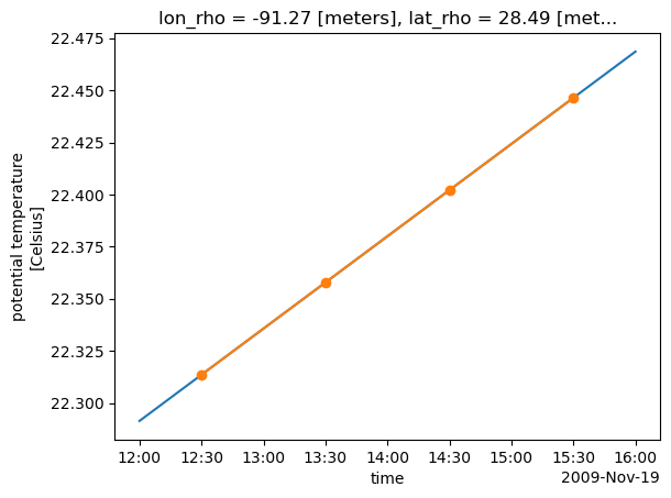
Interpolating in time is straight-forward because it is 1D, uncoupled from the other dimensions. So, we can just use the xarray interp function directly with the desired times. The result is [ocean_time x s_rho x eta x xi].
Notes:
The potentially tricky part is that chunking cannot occur in the direction of interpolation. So, here we reset the chunking and chunk in a different dimension before interpolation, then chunk back to
ocean_timeafterward.You can interpolate in time on the whole Dataset or a single DataArray. The example shows interpolation in time on a single DataArray.
The interpolation times can be sequence-like, but I recommend putting them into a DataArray as follows and demonstrated in the example so that attributes are appropriately added and
cf-xarrayworks afterward (also used in the other interpolation routines).
t0s = xr.DataArray(t0s, dims=’ocean_time’, attrs={‘axis’: ‘T’, ‘standard_name’: ‘time’})
Example usage for a DataArray da:
da.interp(ocean_time=t0s)
# times to interpolate to
startdate = pd.Timestamp(ds.cf["T"][0].values)
t0s = [startdate + pd.Timedelta('30 min') + pd.Timedelta('1 hours')*i for i in range(4)]
# not necessary to change t0s to be a DataArray, but then we can add
# attributes that keep cf-xarray working
t0s = xr.DataArray(t0s, dims=ds.cf["T"].name, attrs={'axis': 'T', 'standard_name': 'time'})
varin = ds.temp
# rechunk from time to vertical dimension
varin = varin.chunk({'ocean_time': -1, 's_rho': 1})
# interpolation
varout = varin.interp(ocean_time=t0s).chunk({'ocean_time':1, 's_rho': -1})
Results are demonstrated below for a single location.
varin.cf.isel(Z=-1, Y=50, X=100).plot()
varout.cf.isel(Z=-1, Y=50, X=100).plot(marker='o')
[<matplotlib.lines.Line2D at 0x76ae04c13a40>]
multiple lon, lat locations (1D)
Function xroms.interpll wraps xESMF so that the wrapper can take care of some niceties. It takes in longitude/latitude values and interpolates a variable onto the desired lon/lat positions correctly for a non-flat Earth. It has functionality for returning pairs of points (1D) vs. 2D arrays of points. First we demo the 1D output.
The result is dimensions [ocean_time x s_rho x locations].
Notes:
Cannot have chunks in the horizontal dimensions.
1D behavior is the default for
xroms.interpllbut also accessible by inputtingwhich='pairs'.Input longitude and latitudes (below
lon0andlat0) can be lists or ndarrays.
Example usage for a DataArray da:
xroms.interpll(da, lon0, lat0, which=’pairs’)
or with xroms accessor:
da.xroms.interpll(lon0, lat0, which=’pairs’)
# use advanced indexing to pull out individual pairs of points to compare with
# rather than 2D array of lon/lat points that would occur otherwise
ie, ix = [24, 100, 121, 30], [31, 198, 239, 142]
varin = ds.salt
indexer = {varin.cf["X"].name: xr.DataArray(ix, dims="locations"), varin.cf["Y"].name: xr.DataArray(ie, dims="locations")}
lat0 = varin.cf["latitude"].isel(indexer)
lon0 = varin.cf["longitude"].isel(indexer)
varcomp = varin.isel(indexer).cf.isel(T=0, Z=-1)
varout = xroms.interpll(varin, lon0, lat0, which='pairs')
assert np.allclose(varout.isel(ocean_time=0, s_rho=-1), varcomp)
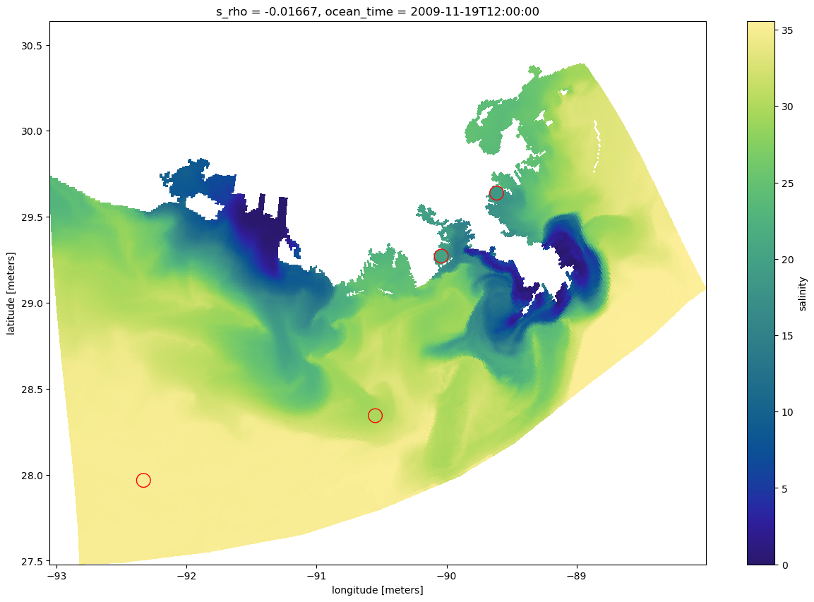
Plot the interpolated surface salinity overlaid on the full field to visually check.
indexer = {'ocean_time': 0, 's_rho': -1}
salt = varin.isel(indexer)
vmin = salt.min().values; vmax = salt.max().values
fig, ax = plt.subplots(1, 1, figsize=(15,10))
salt.cf.plot.pcolormesh(x='longitude', y='latitude', infer_intervals=True, cmap=cmo.haline)
ax.scatter(lon0, lat0, c=varout.isel(indexer), s=200, edgecolor='r', vmin=vmin, vmax=vmax, cmap=cmo.haline)
<matplotlib.collections.PathCollection at 0x76adf74b5be0>
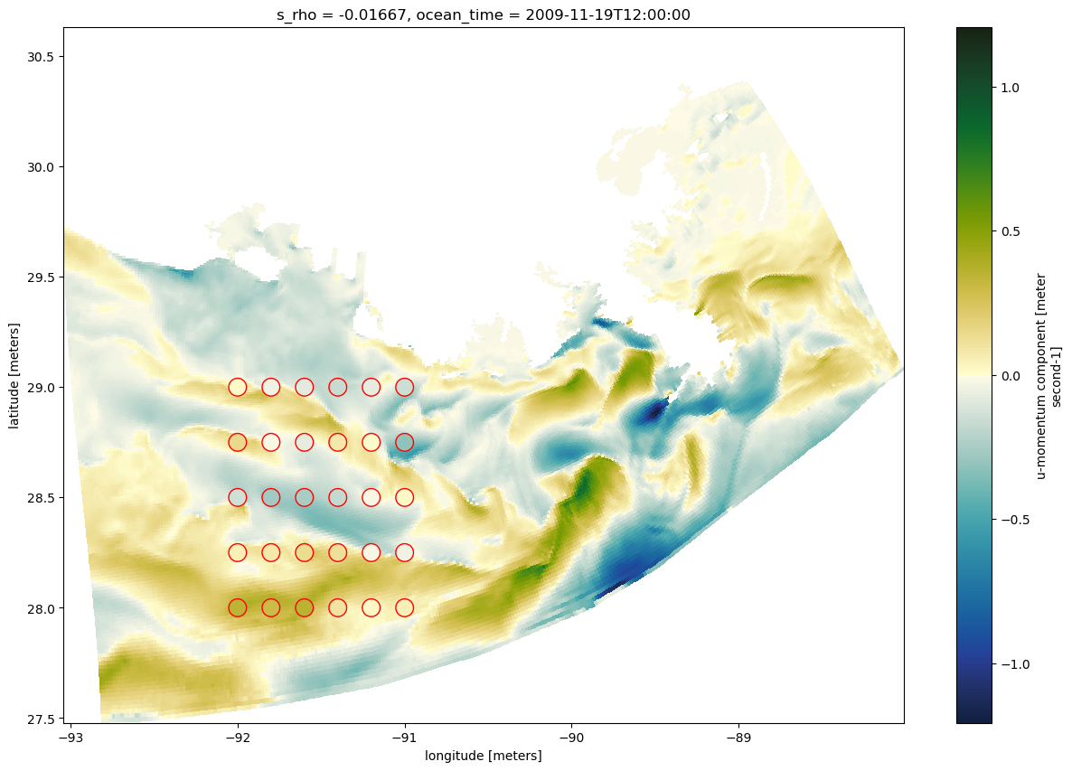
array of lon, lat locations (2D)
We can also use xroms.interpll to interpolate to a 2D grid of longitudes and latitudes.
Result is [ocean_time x s_rho x lat x lon].
Notes:
Cannot have chunks in the horizontal dimensions.
2D grids of lon0, lat0 are found by inputting
which='grid'.Input longitude and latitudes (below
lon0andlat0) can be lists or ndarrays.
Example usage for a DataArray da:
xroms.interpll(da, lon0, lat0, which=’grid’)
or with xroms accessor:
da.xroms.interpll(lon0, lat0, which=’grid’)
npts = 5
lon0, lat0 = np.linspace(-92, -91, npts+1), np.linspace(28,29,npts) # still input as 1D arrays
LON0, LAT0 = np.meshgrid(lon0, lat0) # for plotting
varin = ds.u
varout = xroms.interpll(varin, lon0, lat0, which='grid')
Plot to visually inspect results.
indexer = {'ocean_time': 0, 's_rho': -1}
vmin = abs(varin).min().values; vmax = abs(varin).max().values
vmax = max(vmin, vmax)
fig, ax = plt.subplots(1, 1, figsize=(15,10))
varin.isel(indexer).cf.plot.pcolormesh(x='longitude', y='latitude', infer_intervals=True, cmap=cmo.delta)
ax.scatter(LON0, LAT0, c=varout.isel(indexer), s=200, edgecolor='r', vmin=-vmax, vmax=vmax, cmap=cmo.delta)
<matplotlib.collections.PathCollection at 0x76adf73c3740>
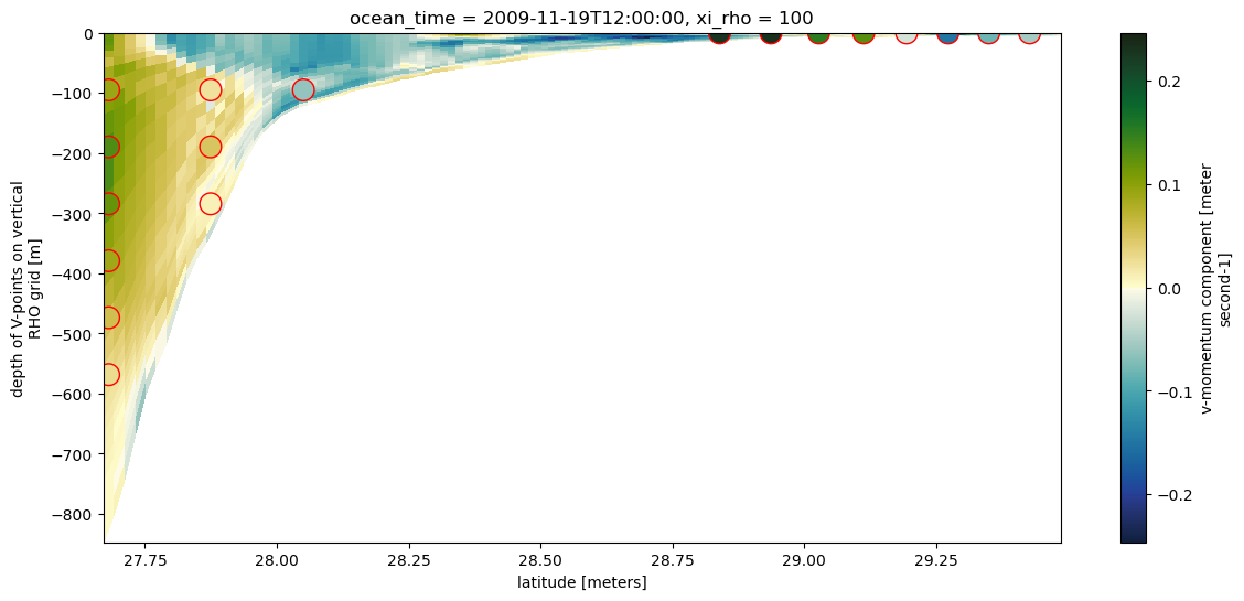
variable regridded to fixed depths
Function xroms.zslice wraps xgcm grid.transform so that the wrapper can take care of some niceties. It interpolates a variable onto the input depths.
The result is dimensions [ocean_time x [z coord] x eta x xi], where [z coord] is the z coordinate used to interpolate the variable to.
Notes:
Cannot have chunks in the vertical dimension.
Input depths can be lists or ndarrays.
xgcm grid.transformhas more flexibility and functionality than is offered throughxroms.zslice; this function focuses on just depth interpolation.Interpolation to fixed depths can be done using time-varying depths or with constant depths in time; do the latter to save computation time if accuracy isn’t very important.
with z varying in time
Use the z coordinates associated with the DataArray in the interpolation.
Example usage for a DataArray da:
xroms.isoslice(da, depths, grid, z=z, axis=”Z”)
More is pre-selected if you used the xroms accessor, with a different name of “zslice”. With DataArray, need to provide grid:
da.xroms.zslice(grid, depths)
With Dataset accessor need to provide DataArray name:
ds.xroms.zslice(varname, depths)
varin = ds.v
varout = xroms.isoslice(varin, np.linspace(0, -600, 20), xgrid)
Plot to visually inspect results:
fig, ax = plt.subplots(1, 1, figsize=(14,6))
dss = varin.cf.isel(X=100, ocean_time=0)
dss.where(~dss.isnull().compute(), drop=True).cf.plot(x='latitude', y='vertical', cmap=cmo.delta)
vmin = abs(dss).min().values; vmax = abs(dss).max().values
vmax = max(vmin, vmax)
toplot = varout.cf.isel(T=0, X=100, Y=slice(None,None,10), Z=slice(None,None,3))
X, Z = np.meshgrid(toplot.lat_v, toplot.z_rho_v)
ax.scatter(X, Z, c=toplot, s=200, edgecolor='r', vmin=-vmax, vmax=vmax, cmap=cmo.delta)
<matplotlib.collections.PathCollection at 0x76adf756c770>
z constant in time
Input separate z coordinates z0 that don’t vary in time for the DataArray to be interpolated to.
Example usage for a DataArray da:
xroms.isoslice(da, depths, grid, z=z0, axis=”Z”)
More is pre-selected if you used the xroms accessor, with a different name of “zslice”. With DataArray, need to provide grid:
da.xroms.zslice(grid, depths, z=z0)
With Dataset accessor need to provide DataArray name:
ds.xroms.zslice(varname, depths, z=z0)
One complication that is currently necessary is to change the metadata such that z_rho_v0 is recognized as the vertical coordinate for ds.v.
var0 = ds.v
# changes to use z_rho_v0 as vertical coordinate
var0.attrs["coordinates"] = var0.attrs["coordinates"].replace("z_rho_v","z_rho_v0")
var0.z_rho_v0.attrs["positive"] = "up"
var0.z_rho_v0.attrs["standard_name"] = "depth"
varout0 = xroms.isoslice(var0, np.linspace(0, -600, 20), xgrid, iso_array=var0.z_rho_v0)
---------------------------------------------------------------------------
KeyError Traceback (most recent call last)
Cell In[12], line 4
1 var0 = ds.v
3 # changes to use z_rho_v0 as vertical coordinate
----> 4 var0.attrs["coordinates"] = var0.attrs["coordinates"].replace("z_rho_v","z_rho_v0")
5 var0.z_rho_v0.attrs["positive"] = "up"
6 var0.z_rho_v0.attrs["standard_name"] = "depth"
KeyError: 'coordinates'
Plot the difference between the two interpolations as a point to see the difference in accounting for time-varying depths and not.
indexer = {'ocean_time': 0, 'Y': 10, 'X': 250}
varout.cf.isel(indexer).cf.plot(y='vertical', figsize=(6,6), lw=3)
varout0.cf.isel(indexer).cf.plot(y='vertical')
multiple locations, depths, and times
A user can simply use multiple of these approaches one after another to interpolate in more dimensions. There are several considerations for the ordering:
Downsize first
If you are going to interpolate in time, depth, and lon/lat, consider if one of those interpolation steps will result in much less model output, and if so, do that step first. For example, if you will interpolate to 3 data locations in lon/lat but 50 vertical levels, first interpolate in lon/lat before interpolating in z to save time.
Chunking
A DataArray cannot be chunked in the dimension that is being interpolated on. So, in the previous example of interpolating first in lon/lat, the DataArray can have dask chunks in the Z and T directions when calculating the lon/lat interpolation. Then, the DataArray would need to be rechunked so that no chunks are in the Z dimension before interpolating in the Z dimension. Similarly for time. You can check chunks with
da.chunks, specify new chunks withda.chunk({'ocean_time': 1, 's_rho': 5})and reset any individual dimension chunking by passing in -1, or reset all chunks for a DataArray or Dataset withds.chunk(-1).
varin = ds.salt
lons, lats = [-93, -92, -91], [28, 28.5, 29]
zs = np.linspace(0, -50, 20)
startdate = pd.Timestamp(ds.ocean_time[0].values)
ts = [startdate + pd.Timedelta('30 min')*i for i in range(10)]
ts = xr.DataArray(ts, dims='ocean_time', attrs={'axis': 'T', 'standard_name': 'time'})
Since there are only a few lons/lats, I will start with that:
varout = xroms.interpll(varin, lons, lats, which='pairs')
print(varout)
The order of the other two steps probably doesn’t matter too much in this case:
varout
varout2 = varout.interp(ocean_time=ts)
varout3 = xroms.isoslice(varout2, zs, xgrid)
# print(varout3)
Note that cf-xarray still works on this output:
varout3.cf.describe()
Cross-section or isoslice
A cross-section or isoslice can be calculated using xroms.isoslice. A short example is given here, but more examples are given in the xroms.isoslice docs. This is the same function used for interpolating variables to fixed depths as demonstrated earlier in this notebook.
Calculate cross-section of u-velocity along latitude of 27 degrees.
grid = ds.xroms.xgrid
lat0 = 27
varin = ds.u
xroms.isoslice(varin, np.array([lat0]), xgrid, iso_array=varin.cf['latitude'], axis='Y')