import xarray as xr
import xroms
import matplotlib.pyplot as plt
import cartopy
import numpy as np
# import hvplot.xarray
# import geoviews as gv
import cmocean.cm as cmo
import xcmocean
How to plot
This notebook demonstrates how to plot ROMS model output from a planview ($x$-$y$) and an $x$-$z$ cross-section. Static and interactive approaches are shown. The cartopy package is used for managing projections for mapview plots, which also gives many options for input (some shown below).
Note you need version 0.11 of Datashader for rasterizing to work in the interactive plots. (https://github.com/holoviz/hvplot/issues/434)
Load in data
Load in example dataset. More information at in input/output page
ds = xroms.datasets.fetch_ROMS_example_full_grid()
ds, xgrid = xroms.roms_dataset(ds, include_cell_volume=True, include_Z0=True)
ds.xroms.set_grid(xgrid)
ds
<xarray.Dataset> Size: 957MB
Dimensions:     (eta_rho: 191, xi_rho: 300, s_rho: 30, ocean_time: 2, s_w: 31,
                 xi_u: 299, eta_v: 190)
Coordinates: (12/29)
    lon_rho     (eta_rho, xi_rho) float64 458kB dask.array<chunksize=(191, 300), meta=np.ndarray>
    lat_rho     (eta_rho, xi_rho) float64 458kB dask.array<chunksize=(191, 300), meta=np.ndarray>
  * s_rho       (s_rho) float64 240B -0.9833 -0.95 -0.9167 ... -0.05 -0.01667
  * s_w         (s_w) float64 248B -1.0 -0.9667 -0.9333 ... -0.03333 0.0
  * ocean_time  (ocean_time) datetime64[ns] 16B 2009-11-19T12:00:00 2009-11-1...
    lon_u       (eta_rho, xi_u) float64 457kB dask.array<chunksize=(191, 299), meta=np.ndarray>
    ...          ...
    z_rho_v0    (s_rho, eta_v, xi_rho) float64 14MB dask.array<chunksize=(30, 190, 300), meta=np.ndarray>
    z_rho_psi0  (s_rho, eta_v, xi_u) float64 14MB dask.array<chunksize=(30, 190, 299), meta=np.ndarray>
    z_w0        (s_w, eta_rho, xi_rho) float64 14MB dask.array<chunksize=(31, 191, 300), meta=np.ndarray>
    z_w_u0      (s_w, eta_rho, xi_u) float64 14MB dask.array<chunksize=(31, 191, 299), meta=np.ndarray>
    z_w_v0      (s_w, eta_v, xi_rho) float64 14MB dask.array<chunksize=(31, 190, 300), meta=np.ndarray>
    z_w_psi0    (s_w, eta_v, xi_u) float64 14MB dask.array<chunksize=(31, 190, 299), meta=np.ndarray>
Data variables: (12/53)
    angle       (eta_rho, xi_rho) float64 458kB dask.array<chunksize=(191, 300), meta=np.ndarray>
    hc          float64 8B ...
    Cs_r        (s_rho) float64 240B dask.array<chunksize=(30,), meta=np.ndarray>
    zeta        (ocean_time, eta_rho, xi_rho) float32 458kB dask.array<chunksize=(2, 191, 300), meta=np.ndarray>
    h           (eta_rho, xi_rho) float64 458kB dask.array<chunksize=(191, 300), meta=np.ndarray>
    Cs_w        (s_w) float64 248B dask.array<chunksize=(31,), meta=np.ndarray>
    ...          ...
    dV_w_u      (ocean_time, s_w, eta_rho, xi_u) float64 28MB dask.array<chunksize=(2, 31, 191, 299), meta=np.ndarray>
    dV_v        (ocean_time, s_rho, eta_v, xi_rho) float64 27MB dask.array<chunksize=(2, 30, 190, 300), meta=np.ndarray>
    dV_w_v      (ocean_time, s_w, eta_v, xi_rho) float64 28MB dask.array<chunksize=(2, 31, 190, 300), meta=np.ndarray>
    dV_psi      (ocean_time, s_rho, eta_v, xi_u) float64 27MB dask.array<chunksize=(2, 30, 190, 299), meta=np.ndarray>
    dV_w_psi    (ocean_time, s_w, eta_v, xi_u) float64 28MB dask.array<chunksize=(2, 31, 190, 299), meta=np.ndarray>
    rho0        int64 8B 1025
Attributes: (12/29)
    file:              ocean_his_0150.nc
    format:            netCDF-3 classic file
    Conventions:       CF-1.4
    type:              ROMS/TOMS history file
    title:             Texas and Louisiana Shelf case (Nesting)
    rst_file:          ocean_rst.nc
    ...                ...
    compiler_command:  /g/software/openmpi/1.4.3/intel/bin/mpif90
    compiler_flags:    -heap-arrays -fp-model precise -assume 2underscores -c...
    tiling:            016x032
    history:           ROMS/TOMS, Version 3.4, Sunday - December 4, 2011 -  7...
    ana_file:          /scratch/zhangxq/projects/txla_nesting6/Functionals/an...
CPP_options: TXLA, ANA_BSFLUX, ANA_BTFLUX, ASSUMED_SHAPE, BULK_FLUX...Setup for plotting
Use cartopy when plotting with a projection and/or wanting to add context like coastline.
proj = cartopy.crs.LambertConformal(central_longitude=-98, central_latitude=30)
pc = cartopy.crs.PlateCarree()
Using cf-xarray with plots
As described in the select data page, xroms is built to use the cf-xarray accessor to make working with dimensions easier.
See description of a DataArray with
ds.salt.cf.describe()
which returns
ds.salt.cf.describe()
Coordinates:
             CF Axes: * X: ['xi_rho']
                      * Y: ['eta_rho']
                      * Z: ['s_rho']
                      * T: ['ocean_time']

      CF Coordinates:   longitude: ['lon_rho']
                        latitude: ['lat_rho']
                        vertical: ['z_rho']
                      * time: ['ocean_time']

       Cell Measures:   area, volume: n/a

      Standard Names:   depth: ['z_rho']
                        latitude: ['lat_rho']
                        longitude: ['lon_rho']
                      * ocean_s_coordinate_g1: ['s_rho']
                      * time: ['ocean_time']

              Bounds:   n/a

       Grid Mappings:   n/a
/tmp/ipykernel_3046/990108105.py:1: DeprecationWarning: 'obj.cf.describe()' will be removed in a future version. Use instead 'repr(obj.cf)' or 'obj.cf' in a Jupyter environment.
  ds.salt.cf.describe()
From this you know that you can use the cf-xarray accessor to call many typical xarray functions from your Dataset or DataArray by substituting the generic Axes names (X, Y, Z, or T) in place of the specific dimension name on the right side of the Axes description. For example:
ds.salt.cf.sel(X=20, T='2010-1-1')
instead of
ds.salt.sel(xi_rho=20, ocean_time='2010-1-1')
A similar syntax works for isel commands.
You also know from this description that calls that take in coordinates for xarray can be used with their generic coordinate name listed above (longitude, latitude, vertical, time). For example:
ds.salt.cf.plot(x='longitude', y='latitude')
instead of
ds.salt.plot(x='lon_rho', y='lat_rho')
We use these shorter generalized Axes and Coordinates below.
xcmocean for choosing colormaps
The xcmocean accessor can be used when plotting with xarray to automatically choose a “good” colormap for the plot based on the DataArray name and attributes and colormaps from the cmocean colormaps package.
To use the colormap accessor, add .cmo before the plot call from xarray (but skip the plot if specifying the type of plot subsequently, like pcolormesh). These are the call options:
cmo.plot()cmo.pcolormesh()to specifypcolormeshcmo.contourf()to specifycontourfcmo.contour()to specifycontour
ds.v.cf.isel(T=0, Z=-1).cmo.pcolormesh()
<matplotlib.collections.QuadMesh at 0x7478a4c20890>
xcmocean can also be used in conjunction with cf-xarray but with slightly different syntax. You can access the same plot options while using cf-xarray in the plot call with the following:
cmo.cfplot()cmo.cfpcolormesh()cmo.cfcontourf()cmo.cfcontour()
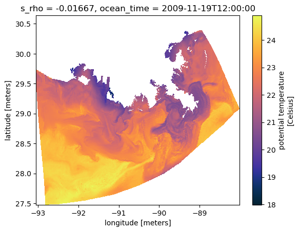
ds.temp.cf.isel(T=0, Z=-1).cmo.cfpcolormesh(x='longitude', y='latitude')
<matplotlib.collections.QuadMesh at 0x7478a4cadb20>
Static: xarray
Can plot directly in xarray since it has wrapped many Matplotlib plotting routines. This is great for quick plots and continues to improve, but if you need more control then try the next section of plotting directly in Matplotlib.
map view
Overview
Plotted with dimension indices instead of coordinates:
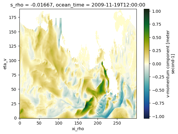
ds.v.cf.isel(T=0, Z=-1).plot(cmap=cmo.delta)
<matplotlib.collections.QuadMesh at 0x74789cf604d0>
Plotted with coordinates lon/lat:
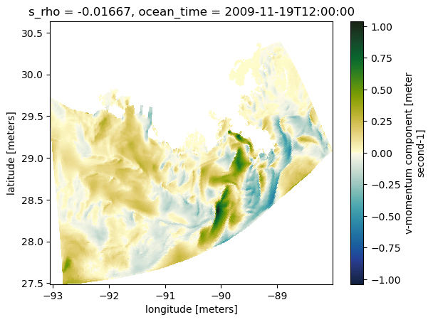
ds.v.cf.isel(T=0, Z=-1).cf.plot(x='longitude', y='latitude', cmap=cmo.delta)
<matplotlib.collections.QuadMesh at 0x74789cf76840>
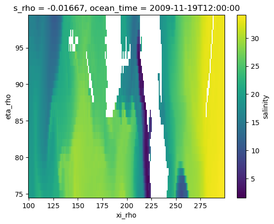
magnified
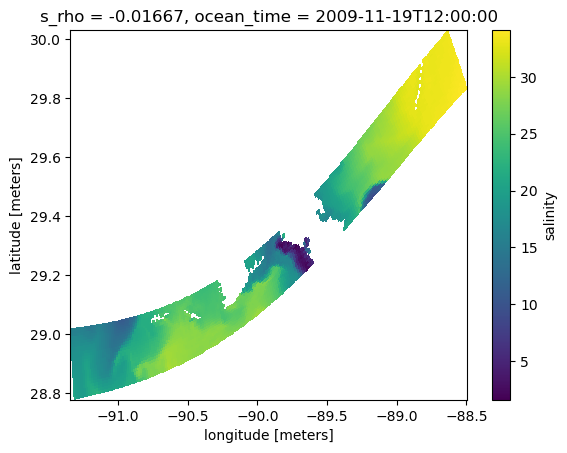
ds.salt.cf.isel(T=0, Z=-1, X=slice(100,300), Y=slice(75,100)).plot()
<matplotlib.collections.QuadMesh at 0x74789c4d6f00>
ds.salt.cf.isel(T=0, Z=-1, X=slice(100,300), Y=slice(75,100)).cf.plot(x='longitude', y='latitude')
<matplotlib.collections.QuadMesh at 0x74789c5b04d0>
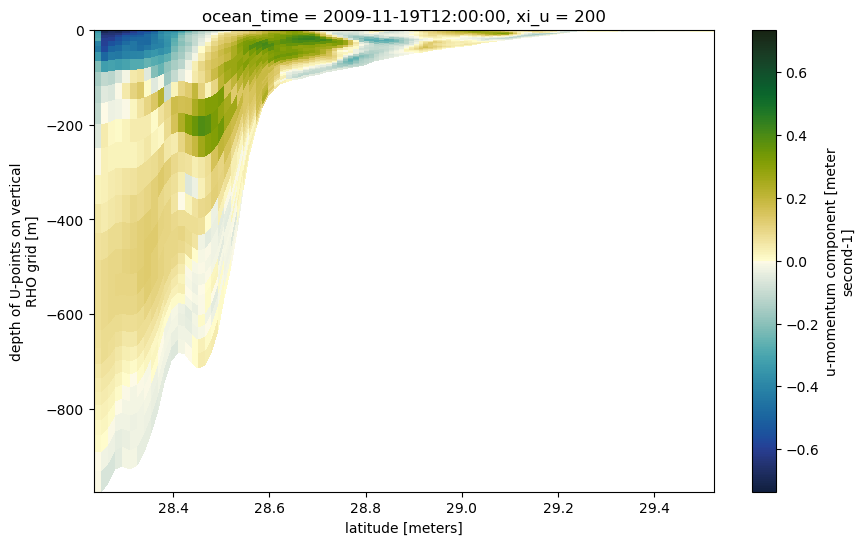
cross-section
dss = ds.u.cf.isel(X=200, T=0)
dss.where(~dss.isnull().compute(), drop=True).cf.plot(x='latitude', y='vertical', cmap=cmo.delta, figsize=(10,6))
<matplotlib.collections.QuadMesh at 0x74789c408260>
Static: Matplotlib
map view
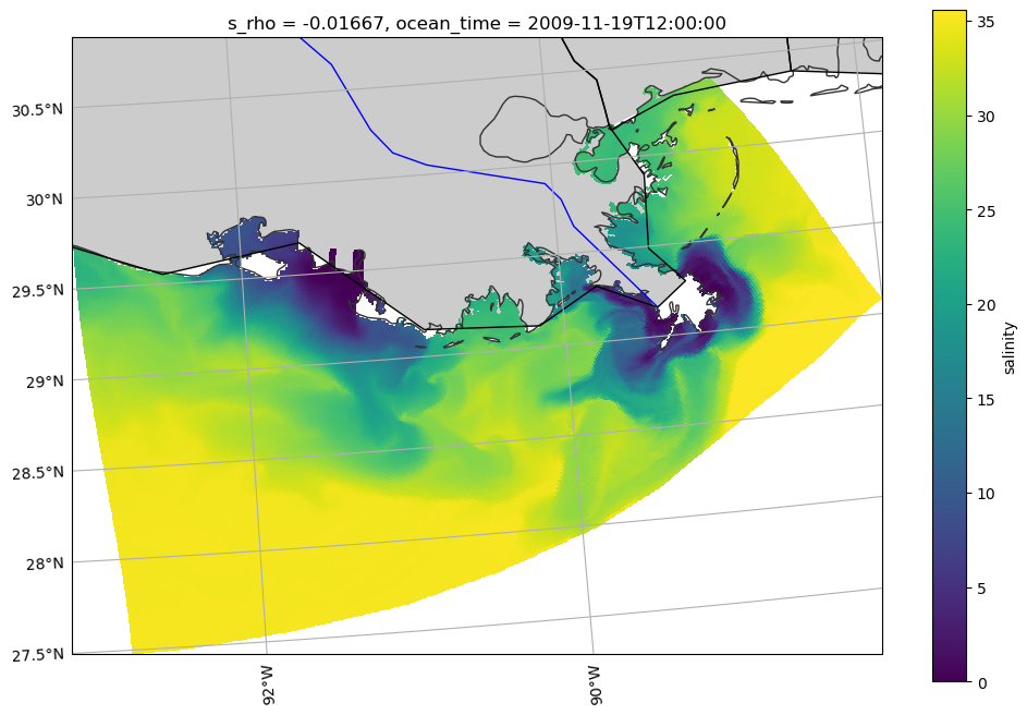
Overview
Here is a basic plan-view map, using cartopy for projection handling. You can add many different types of natural data for context. Shown here are coastline, land, rivers, and state borders. You can control the resolution of the data by changing the input to with_scale (options are ‘10m’, ‘50m’, or ‘110m’, corresponding to 1:10,000,000, 1:50,000,000, and 1:110,000,000 scale). More cartopy feature information available here: https://scitools.org.uk/cartopy/docs/v0.16/matplotlib/feature_interface.html.
fig = plt.figure(figsize=(12,8))
ax = plt.axes(projection=proj)

# Add natural features
ax.add_feature(cartopy.feature.LAND.with_scale('110m'), facecolor='0.8')
ax.add_feature(cartopy.feature.COASTLINE.with_scale('10m'), edgecolor='0.2')
ax.add_feature(cartopy.feature.RIVERS.with_scale('110m'), edgecolor='b')
ax.add_feature(cartopy.feature.STATES.with_scale('110m'), edgecolor='k')

gl = ax.gridlines(draw_labels=True, x_inline=False, y_inline=False, xlocs=np.arange(-104,-80,2))

# manipulate `gridliner` object to change locations of labels
gl.top_labels = False
gl.right_labels = False

ds.salt.cf.isel(T=0, Z=-1).cf.plot(ax=ax, x='longitude', y='latitude', transform=pc)
<cartopy.mpl.geocollection.GeoQuadMesh at 0x74789c3404d0>
/home/docs/checkouts/readthedocs.org/user_builds/xroms/conda/stable/lib/python3.12/site-packages/cartopy/io/__init__.py:242: DownloadWarning: Downloading: https://naturalearth.s3.amazonaws.com/110m_physical/ne_110m_land.zip
  warnings.warn(f'Downloading: {url}', DownloadWarning)
/home/docs/checkouts/readthedocs.org/user_builds/xroms/conda/stable/lib/python3.12/site-packages/cartopy/io/__init__.py:242: DownloadWarning: Downloading: https://naturalearth.s3.amazonaws.com/10m_physical/ne_10m_coastline.zip
  warnings.warn(f'Downloading: {url}', DownloadWarning)
/home/docs/checkouts/readthedocs.org/user_builds/xroms/conda/stable/lib/python3.12/site-packages/cartopy/io/__init__.py:242: DownloadWarning: Downloading: https://naturalearth.s3.amazonaws.com/110m_physical/ne_110m_rivers_lake_centerlines.zip
  warnings.warn(f'Downloading: {url}', DownloadWarning)
/home/docs/checkouts/readthedocs.org/user_builds/xroms/conda/stable/lib/python3.12/site-packages/cartopy/io/__init__.py:242: DownloadWarning: Downloading: https://naturalearth.s3.amazonaws.com/110m_cultural/ne_110m_admin_1_states_provinces_lakes.zip
  warnings.warn(f'Downloading: {url}', DownloadWarning)
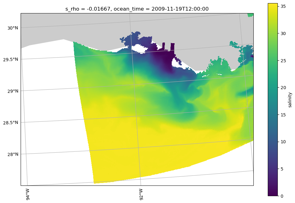
Magnified
Use set_extent to narrow the view to magnify a subregion.
fig = plt.figure(figsize=(12,8))
ax = plt.axes(projection=proj)

ax.set_extent([-94, -90, 27.5, 30], crs=pc)
ax.add_feature(cartopy.feature.LAND.with_scale('110m'), facecolor='0.8')
gl = ax.gridlines(draw_labels=True, x_inline=False, y_inline=False, xlocs=np.arange(-104,-80,2))

# manipulate `gridliner` object to change locations of labels
gl.top_labels = False
gl.right_labels = False

ds.salt.cf.isel(T=0, Z=-1).cf.plot(ax=ax, x='longitude', y='latitude', transform=pc)
<cartopy.mpl.geocollection.GeoQuadMesh at 0x74789c5955e0>
cross-section
This is the same as the example above for plotting directly from xarray since projections on plan-view maps make most of the difference.
dss = ds.u.cf.isel(X=200, T=0)
dss.where(~dss.isnull().compute(), drop=True).cf.plot(x='latitude', y='vertical', cmap=cmo.delta, figsize=(10,6))
<matplotlib.collections.QuadMesh at 0x7478a4e227e0>
Interactive
In these interactive plots, you can zoom, pan, and save plots using the menu on the right-hand side. There is a mouse hover option to display specific values; this can also be turned off. The plot automatically makes a widget to the right of the plot to easily vary over that variable. Currently the plots below are set to vary over time.
These plots aren’t working interactively in the docs, but are left here as examples for your own use.
map view
The tiles allow for different basemap options. The rasterize option is really important here by allowing a lower resolution presentation when zoomed out and increasing resolution with magnification, potentially saving a lot of time.
Vary over time (for surface)
tiles = gv.tile_sources.ESRI  # optional, for a basemap
ds.salt.cf.isel(s_rho=-1).hvplot.quadmesh(x='lon_rho', y='lat_rho', width=650, height=500,
                        cmap="cmo.haline", rasterize=True, crs=pc) * tiles
Vary over sigma level and time
tiles = gv.tile_sources.ESRI  # optional, for a basemap
ds.salt.hvplot.quadmesh(x='lon_rho', y='lat_rho', width=650, height=500,
                        cmap=cmo.haline, rasterize=True, crs=pc) * tiles
Vary over depth and time
Since the vertical dimension is in sigma coordinates instead of fixed depths, it is not immediate to be able to use a widget to vary depth in these plots. However, it is still possible to do using xroms code. First set up the calculation for several depths you want to examine using xroms.isoslice, then send that xarray object to hvplot for plotting. It is slow because it has to calculate everything, but it is nevertheless interactive. Having these files locally would speed it up.
In the following example, we use the accessor version of the isoslice interpolation to find slices of salinity at fixed depths. To save some time, we use the time-constant depths (z_rho0) associated with salinity instead of the time-varying version (z_rho).
zsalt = ds.salt.xroms.isoslice([-10, -20, -30], iso_array=ds.salt.z_rho0, axis='Z')
tiles = gv.tile_sources.ESRI  # optional, for a basemap
zsalt.hvplot.quadmesh(x='lon_rho', y='lat_rho', width=650, height=500,
                        cmap=cmo.haline, rasterize=True, crs=pc) * tiles
cross-section
In this case, the plots are similar whether rasterize=True is used or not.
ds.temp.isel(xi_rho=300).hvplot.quadmesh(x='lat_rho', y='z_rho0', width=750, height=400,
                        cmap=cmo.thermal)